Power Prediction of VLSI Circuits Using Machine Learning

1  Introduction to Power Estimation

Industrial testing is a crucial element of the project development phase of the microchip. Its objective is to discover faulty gadgets and to straighten them out. A pre-generated training set is given to every microchip produced [1]. For fast and expense verification, on-chip scanning devices that simulate non-functional working circumstances have been employed extensively. In return, this generates problems of power. Regulatory systems are closely adjusted to suit the strict power requirements for the chip [2]. However, the energy demands are exceeded by non-functional working circumstances employed in the testing process.

That might result in improper test findings and harm to the chip. Tests must thus be reviewed beforehand to verify they comply with power demands to provide safety within the assessment [3]. The IR-drop might create time infringements as an additional problem. Precise simulation techniques need to be used to provide reliable findings before recording within the sign-off phase. However, many rounds can be used by the remedial procedures to minimize the IR loss for every occurrence independently [4]. Sadly, precise energy and schedule calculations need enormous funds and unnecessary runtime. In addition, analyses were only carried out near retransmitting in a later phase in the project [5]. Consequently, it is impossible to finish the modeling of all assessments. Typical choices include a limited sub-set of tests for precise Simulation. This selection ideally includes the worst circumstances possible. The choice of scenario-related tests that contribute to electrical problems during testing is crucial [6].

Initially, a few pre-selected trials are replicated precisely like in normal flow. Once a certain test encompassing the worst-case possibilities has been accurately analyzed, it is feasible to have other trials that create power problems [7]. Also, for such designs, the remedial repetition doesn’t always work for others. This study aims at the discovery via forecasting of worst benchmark functions [8]. It suggests that the automated forecasting system prevents the comprehensive analytical evaluation of all training sets from describing the actual energy behavior throughout all experiments. These processes are helpful as training images for training [9]. The testing vectors and the investigation outcomes are subsequently utilized to develop a machine learning (ML) network using the simulating information [10]. This learning algorithm is then utilized to predict the forecast develop materials with no need to simulate explicitly. This technique enables the broad discretion of testing to be predicted. The registration is classified into two parts:

•   The entire (global) energy demand of a testing t is intended and anticipated to identify critical tests.

•   Focused and expected to need tests are the entire (global) power usage of a test t. Because low energy demand cannot ensure the lack of strategic locations, energy use is linked to the processor’s architecture. It can forecast local areas of high.

In comparison with the current effective assessment, the forecast time is quite minimal. Simultaneously, the projected values are extremely dependable and only indicate a tiny difference from the real simulated data [11]. All tests were processed and their related power profile evaluated to detect possibly lethal power testing. Thus, the suggested strategy enhances the total opportunity for essential testing throughout the start-up period.

The primary contributions of this article are as follows:

•   The suggested approach can manage the alteration of macro/cell blocks, the change of structures, and the adjustment of power circuits without recertification of a model.

•   The technique enables flexibility as the specific set collection for proprietary product nodes and the sub-group of metallization irrespective of architecture, power grid, and cellular library sizes.

•   It offers criteria that allow users to select while starting new tools to upgrade a training set.

The remainder of the paper is as follows: Section 2 describes the background to the energy prediction models. The proposed machine-based circuit power estimation (ML-CPE) system is designed and implemented in Section 3. Section 4 discusses the software analysis and evaluation. The conclusion and future scope of the proposed system are depicted in Section 5.

2  Background to the Energy Prediction Models

Unlike any other on-chip device, a continuous famine for power became a fact every two years. The power issue grew worse, reducing the size of various processing nodes. The load demand helped solve the growth of which depended heavily on the shrinkage of a base station. Thus, it concluded a more exact energy demand prediction model was necessary to differentiate static elements from movements suggested by Shanmugham et al. [12]. Complementary metal-oxide-semiconductor integrated circuit (CMOS IC) offered an overview of power loss through a correct power analytical technique, enabling programmers and integrated circuit (IC) architects to produce better resource-accurate alternatives. There were various CMOS IC electricity options [13]. However, few offered precise distinguishing among steady and dynamic heat removal elements. A technique for such power assessments was the answer given in this study. The relevance of the difference among stable and dynamical elements was not considered in actual assessments suggested by Abbassi et al. [14]. The power taken by the procedure during the implementation was observed to get the basic cost of command. The debate about the deconstruction of observed into stationary and non-stationary elements was neglected [15]. It was seen that cross effects could be ruled out due to a minimal impact on daily expenditure, which wasn’t the situation with the particular platform employed in this study, that in some instances surpasses the initial expenses many times, depending on such impact.

The provided energy consumption identified numerous nuclei, with several major changes, like the version described in this study suggested by Palma et al. [16]. First and foremost, the methodology is applied to diverse multi-core devices and assesses energy at command instead of resource use. The big distinction between the framework mentioned here and those introduced was that it unlikes the designs given in this chapter which covered all facets of electricity consumption, kinematic and dynamic suggested by Khana et al. [17]. The assessment framework kept track of only the dynamic electricity usage of several core processing units.

The research introduces state-of-the-art measuring devices capable of measuring energy spent across two phases. However, there was still no proper debate on measuring active and passive energy suggested by Ashok et al. [18]. The suggested energy demand estimate model incorporated static power as a separate model component. The model was tested with the central processing unit (CPU) core ARM7. Yet, the static energy technique or practical implications for the element evaluated in the goal core have not been properly stated [19]. The suggested model was validated. Just short recovery values were validated, which might not be the situation in the study described in this document. Provided techniques for estimating power usage are dependent on the operating system of emulation, and hence the intended architecture for such a study cannot be utilized [20]. Static power was pushed in the scientific work as one of the factors inside the estimated power consumption framework. After verification testing was started at various clock rates, the issue arose. Verification tests have failed due to false static energy compared to the major reason for this study suggested by Fahd et al. [21].

Methods for forecasting the waste of energy of programming code were described at a logical level. The batch processing system’s energy calculation was extremely imprecise owing to its protocol layer for varied uses. Statistical approaches were described for the estimation of peak loss. Additional work provided the register-transistor-logic (RTL) forecast of changing data using predictive methods suggested by Shavali et al. [22]. Unlike previous approaches, the study focused on the network level forecast employed throughout the semiconductor design sign-off phase. Monte-Carlo-based techniques and other analytical techniques said the average energy was less reliant on simulations and required less time to calculate the mean operational energy. These earlier approaches cannot, though, be utilized to forecast the proposed method consists that was very high compared to the operational energy [23]. Following a project change request, the IR decline was predicted using a newly suggested machine learning (ML) based approach, utilizing simulation data produced. In Addition, test models were included in the set of features utilized in the technique presented. Artificial very large scale industry (VLSI) energy estimated network-based approaches yield good accuracy with a specified net architecture. Active learning (AL) necessitates a close relationship between the developer and the machine. The machine selects one or more things from an unlabeled training set at each cycle of the learning process, and the developer identifier [24].

3  Proposed Machine-Based Circuit Power Estimation System

A parasite estimating engine has just been created to solve the difficulties described in the preceding section. It uses Machine Learning Technology to train estimate models and forecast parasites with focuses on issues extracting information. For pre-routing temporal forecasting in the online world, machine learning was proposed. It is used a convolutional neural network (CNN) model in the parasite estimation process. A pre-layout network is converted together into a multi-port Series circuit having extracted interconnected parasitism. This change takes place in all networks of a circuit which subsequently results in pre/post computation to substantial variations. It utilizes a surrogate for a floor plan circuit to predict the Converter for every pre-layout structure.

3.1 Modeling

The architecture and connectivity of any network might be unique from everyone else. It estimates every post-lay-out system with multiple scalars, efficient capacitors, and impedance to trace the issue with deep learning. Useful capacitor Cae is the total—such as grounded and cross capacities to other networks–of the enable continuous encountered on the network. It utilizes a continuous-time network model to compute active resistance. Now it establishes the idea of an efficient temporal constant that considers the time constant of an initial electrical system. An efficient process takes given for the network with N poles po1,po2,…,pon. The effective learning process is denoted in See Eq. (1)

∝e=1po12−1+1po22−1+⋯+1pon2−1(1)

The power of the individual component is denoted pox. All the powers are squared and then taken root, and the inverse of all th powers and their summation results shows the effective learning rate.

The pictorial representation of αe is depicted see Fig. 1 above. That enables more effective impedance to be calculated using See Eq. (2)

Ree=αeCae(2)

The effective learning rate is denoted αe, and the effective capacitance is depicted Cae. Only by adopting the basic star topology illustrated. The branch resistance is denoted Rebr=ReeN. The star network has a step response equal to the efficient post-layout overall time characteristic. Where N is the amount of transistors links to the network, could synthesize a post-lay-up network’s efficient impedance and inductance.

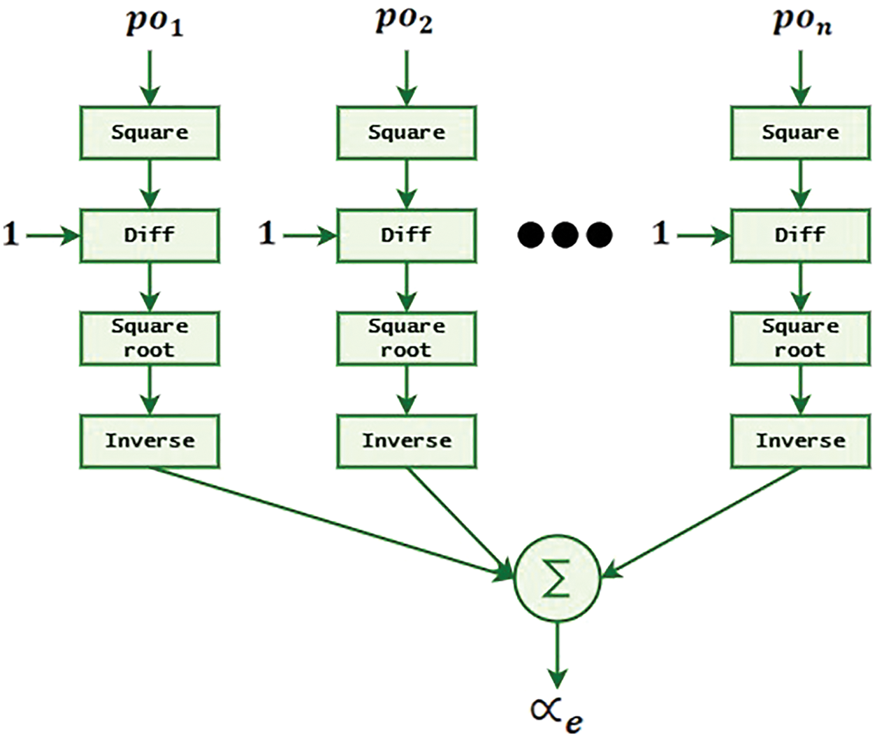
Figure 1: Pictorial representation of αe

3.2 Power Analysis

The ML technology is suggested to anticipate the action of all training set at the international and national levels to save time. International action corresponds to the sum energy of the trial for our research, whereas local action corresponds to the trial energy in terms of the design. Functionality and testing datasets are the key elements for the usage of machine learning. Features must be gathered from local phases of flow rate for the real power estimation and dispersion across the structure.

The workflow of the proposed ML-CPE system is depicted See Fig. 2. It uses a netlist from the components. The filtered netlist is used for feature extraction. The final predicted energy consumption of the circuit is calculated and shown in the output files. Data relating to design are accessible in several types, used by various technologies, and handled properly. In such folders, the data is necessary for many purposes. For such a learning component, the necessary data must be retrieved and presented. It shows the creation of the given data and the separation of training method functions. The data required are as follows:

Figure 2: Workflow of the proposed ML-CPE system

3.2.1 Design Information

In the technique, the necessary data are retrieved from automatic test records and saved for future analysis, i.e., the substance of the scanning cells in such a transition and grab function for every scan chain and perform a thorough.

3.2.2 Simulation and Analysis

Displacement and recording of the performed trials lead the logic components of the system to be active. It simulates the training examples by doing the exercise. This data is captured and also can, after simulations, be saved, a different format file describing logical value changes across discrete times. Remember that logic simulations do not generally analyze data on equipment and hence do not give energy usage data. The modeling data must be evaluated with appropriate cell and technique information to generate the power requirements for a simulation experiment. That is the portion that takes time and resources. It shows the design and simulation findings when simulation data is accessed for a test sequence. This information is retained for testing purposes following the statistical method.

The hardware module of the proposed ML-CPE system is depicted See Fig. 3. It has several ports and modules for interconnectivity. Technology is used to denote the component size, gate level data from each component is collected, and then the test parameters, location, and layers are fed to the prediction model to calculate the energy prediction of the circuit.

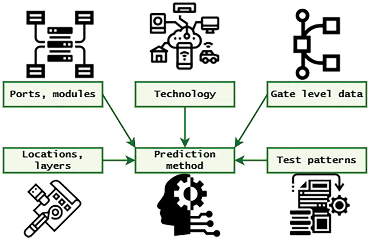
Figure 3: Hardware model of the proposed ML-CPE system

3.2.3 Technology and Physical Layout

The gateways’ actual position and other design information are not needed for the objective of worldwide energy usage alone. However, this information is analyzed and stored for local problem areas to be identified. The position and dimension of cells are retrieved throughout the design data. This data is input in market Design tools or alternative techniques, such as base maps, to discover energy regions.

3.3 Machine Learning Model

To forecast the test power requirements, it employs trained ML techniques. For the generation and training of the model structure, the information and characteristic extracts are employed.

3.3.1 Linear Least-Square Regression (LLSR)

LLSR is a fundamental and commonly used computer modeling approach. The LLSR approach produces a model for the estimated variable using the linear estimate methodology. The b=(b1,b2,…,bn) coefficients are reduced to the minimum among the anticipated calculated and the results. The inaccuracy of the expected value is minimized during the training stage. i.e., the target is stated in Eq. (3)

minimum(|Vb−C|2)(3)

If the vector V is unique, the resulting model is vulnerable to random mistakes. The bias condition is denoted b, and the correlation is denoted C. The parameters of the solution are regardless of the relevance to measuring. Where there are linear relationships within the factorial design V column owing to correlated factors, the issue of multicollinearity arises. That allows for a huge inaccuracy when several values are predicted.

3.3.2 Ridge Regression

The Ridge Reconstruction technique was proposed to decrease the inaccuracy of LLSR oriented approach. A further error compensation parameter is utilized here. The extra parameter called the rim coefficient lowers the mistake by placing a punishment just on factor size. The calculation is expressed in Eq. (4)

minimum(|Vb−C|2+φ|b|2)(4)

where φ is the variable of adjustment that checks the penalizing intensity, the vector is denoted V, the bias condition is denoted b, and the correlation coefficient is denoted C.

3.3.3 K-Nearest Neighbors Regression (K-NNR)

The above-stated parametric prediction models are challenging to moderate. It also employed a non-parametric method, the analysis K-Nearest Neighborhood (KNNR), that recognizes the oscillation of Tro, that is closest to the pro forecast point. The ultimate value, i.e., X(pro), is estimated even more by summing the answers about Tro. The official description should be provided in Eq. (5)

X(pro)=1M∑i=0Troci.(5)

M optimal value relies on a tradeoff between imbalanced data. M can be provided or approximated throughout the performance. the correlation is denoted ci. A low ratio of M usually gives a big difference, and conversely.

3.3.4 Neural Network Regression

The aim was to improve the precision of the forecast result by proposing a computer vision learning technology, termed Multi-Layer Perceptron (MLP). The non-linearities are buried among the endpoints in this estimation method. The MLP-based training model calculates a functional g(.)=Vin→Vout. Where in represents the analysis of complex and out outcome variables. If the machine learning model is labeled, i.e., have both the a=(a1,a2,…,am) Attribute and a goal, MLP can forecast a non-linear regression technique.

3.4 Measurement Model

To compute another element, distinguished observation of stability and energy loss requires an evaluation. In the case of disabling clock dispersion with the whole CMOS IC, the dynamical energy dissipation can be eliminated; however, that isn’t the scenario for many targeted systems. It just has a way to test that, even if it can shut off clock dissemination. This study used the ultra-low energy heterogeneity digital signal processing (DSP) structure of the proposed intended for hearing devices. The technological manufacturing unit was designed utilizing 90 nm. There are five distinct DSP nuclei. One DSP core acts to control and coordinate physical events like a microprocessor. For diverse operations, two DSP components are generally useful. The other two DSP units are developed and tuned to accelerate numbers. In addition, the I/O interface, the reciprocal sync, and the scalability of amplitude and current are based on numerous peripherals.

Appropriate numerical configurations like clock rate and dispersion, power scaling, specific function registries (SFR), etc., must be downloaded to set up a particular system for experiments. The measurement model of the proposed system is depicted in Fig. 4. It uses both training and testing data from the database. The necessary features are extracted from the machine learning model, and the final predicted energy is produced as the final output. It is crucial to note that such a targeted system can nearly fully disable clock dissemination.

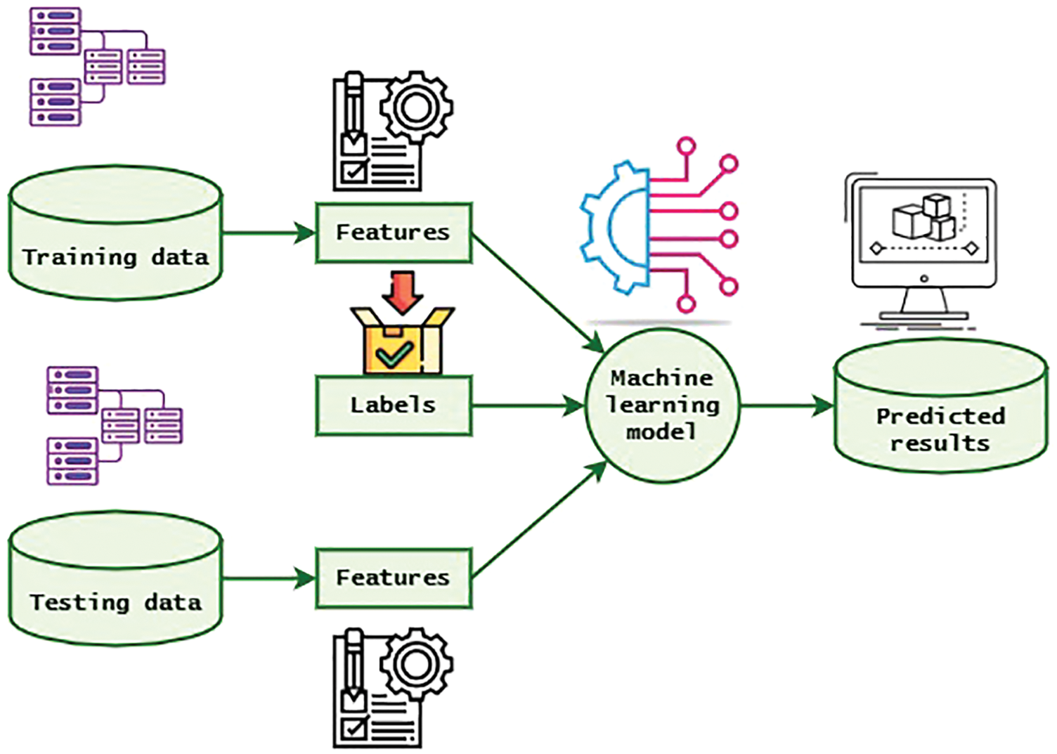
Figure 4: Measurement model of the proposed system

3.5 Simulation Results

The simulation model and the necessary steps for the Simulation are discussed in this section. Networks of convolutional neural network (CNN) for many training methods, variables like training data, epoch, hidden units, and impetus constants vary. A four-layer convolutional neuro propagating framework is designed. The first level with a “regular” Converter is set, while the subsequent levels select a “transit” function. Nine characteristics comprise the library of circuit design. Thus the amount of parameters for the system is nine. Two phases constitute the suggested Artificial System energy estimate technique. The system is designed in the first stage, and also the system test can also be performed as in the second step. The following stages are addressed in the learning phase.

3.5.1 Training Phase

Step 1: The training is performed using input variables taken from ISCAS’89 circuitry.

Step 2: Every one of the original input parameters is normalized with its respective goal vectors. The limit of normalization for the hidden secondary level, the third convolution layers, and the suggested hidden layers are −1 to +1 whenever the artificial neuron selected for such cells is Tan-sig. The normalization band is 0 to 1. A third deep learning model and output vector of the suggested CNN is a File for the selected activating module for neurons with just one concealed layer. Standardization for CNN is carried out from −1 to +1.

Step 3: The neural networks are trained using standardized input variables and matching standard target variables.

3.5.2 Testing Phase

Step 1: Testing is done using input data left out during the training phase.

Step 2: Incoming test matrices also standardized the various criteria the same way as normalization in training.

Step 3: For these normalized test input data, the system creates standardized convolution layers.

Step 4: Normalised output matrices are transformed to their initial amount by implementing the reverse normalization procedure.

Step 5: The outcome vectors generated for such test sources are contrasted and validated by the linear regression with predicted results.

3.5.3 Application

The problematic formulation is described as follows as a pedagogical approach. A test vector n is a logical sequence {0, 1 }. A group of matrices is being used to educate a model g as indicated above Trn. For this tiny selection, a simulation is performed to provide a power usage of every test. The suggested technique employed the weighted action of changing prediction models or more precise heat removal metrics. Classifier g is trained with simulated results. The first use is to anticipate the worldwide power distribution. The first use is power rating is a factor (Ptr), and it is expressed in See Eq. (6)

Ptr=b1(t1)+b2(t2)+⋯+bn(tn)(6)

When the variables b1,b2,…,bn .are the metric energy values for the node d1,d2,…,dn respectively. The data are collected by precise (time-consuming) computation of trained training examples.

Dure training includes a function gk that predicts, dependent on the logical contents of network input neurons Ptr, the scanning cells withi gk n the learning method, which is employed as a box. The predicted power function is denoted in Eq. (7)

gk(Ptr)=g(m1,m2,…,mk)(7)

At which input power nodes is m1,m2,…,mk. That is accomplished during the training with the continual refining of gk(Ptr). Er is intrinsically expressed as Ery(x)=try(x)−pry(x), where Er denotes the real result of the learning and pr as a projected result of the node. To reduce the gap between the predicted number and the actual number, by modifying load, a mathematical programming function for gk(Ptr) is performed as per the training method employed. After the testing period, the gk(Ptr) the function used to forecast its power requirements depending on the taught gk(Ptr) for other training examples. The second trial is the electric supply forecast over the design (local power). The component i,j coordinates as in layout must be incorporated in the teaching and learning activity to use the learning techniques. The final predicted energy of the circuit is given in Eq. (8)

gn(Ptr(i,j))=g(b1(i1,j2),b2(i2,j2),…,bm(im,jm)(8)

The position of a node m is thus substituted (i,j). The biasing condition is denoted bx(ix,jx). By doing so, the circuit architecture is considered to anticipate every node’s action. The testing vectors are trained and predicted similarly to those described previously. The result of the forecasting procedure is the location-related changing action. The offline files anticipated then are normally described as the exact source data in the testing process. That can be added to design tools, or grouping methods wherein hot areas depending on computed data are recognized.

3.5.4 Inference

While it developed a design, it utilizes it to prevent pre-layout graphical network interconnected parasites that have not previously been observed. The layout output is first analyzed, and the functions of each Net are extracted. Next, those characteristics gave to a training randomized forests model Ree and Cae. It synthesizes a network system for every network to use these primitives. In analog design, paramilitary matching is crucial to decrease variance in certain dynamic circuits. That illustrated graphical form provides estimated parasite data in the Standard Parasite Exchange File (SPEF).

4  Software Evaluation

With this package of sci-it-learn, it developed a model training in Python. It utilized analog blocks 202 and 627 for a system, correspondingly, to learn 18 and 4 nm. There is a range of commercial circuit applications in the 18 nm and 4 nm databases. It initially used the architecture files for backups as focused on data collection. Then, it gains Ree and Cae Worth from prior post-layout structure that was then employed for the Randomized Forests network training. It is crucial to highlight that the system doesn’t rely on stimulus testing tables. It has already been utilized for gathering information and modeling with minimum change to the whole flow for numerous distinct manufacturing techniques.

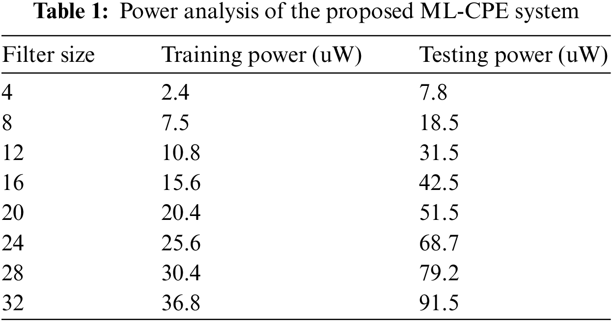
For example, see Tab. 1 indicates the power analysis of the proposed ML-CPE system. The proposed ML-CPE system is designed with the help of a machine learning model such as a convolutional neural network, and it helps to increase the prediction of the system. The proposed ML-CPE system is trained with the variations in the filter size, and the respective power is analyzed. As the filter size increases, the respective utilized power also increases. The accuracy of the proposed ML-CPE system in the testing condition is higher than training condition.

Figs. 5 and 6 show the average absolute error (AAE) and the maximum absolute error (MAE) analysis of the proposed ML-CPE system, respectively. The proposed ML-CPE system is implemented using the dataset, and the system consists of nine different circuits. It is named C1, C2, …, C9. The error analyzed in each circuit is analyzed and plotted for the pre-layout and the proposed ML-CPE system. The proposed ML-CPE system with a machine learning model helps the systems learn the circuits well and produces predicted energy with higher accuracy.

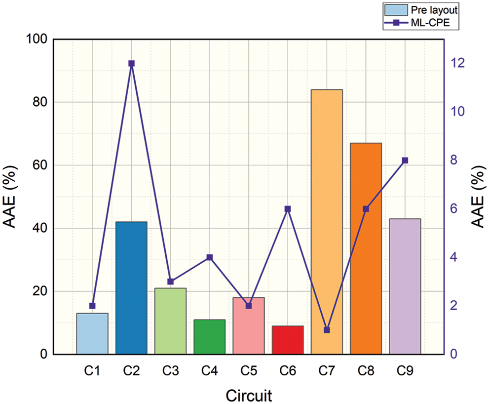
Figure 5: Average absolute error analysis of the proposed ML-CPE system

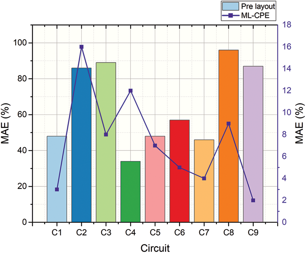
Figure 6: Maximum absolute error analysis of the proposed ML-CPE system

Figs. 7 and 8 show the power analysis of the proposed ML-CPE system’s training and testing conditions, respectively. The simulation analysis of the proposed ML-CPE system is carried out by varying the filter size from minimum size to maximum size. The respective power utilization of the circuit is monitored and plotted. As the filter size increases, the respective power utilization of the circuit also increases. The proposed ML-CPE system with a machine learning model enhances the accuracy in testing conditions with the help of trained data.

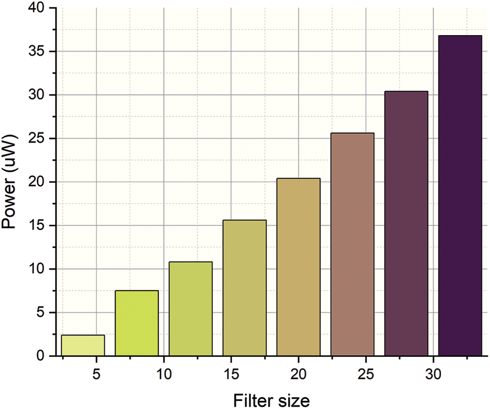
Figure 7: Power analysis of the training condition

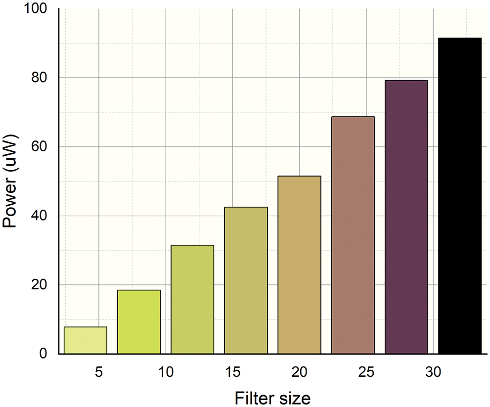
Figure 8: Power analysis of the testing condition

For example, see Tab. 2 shows the error analysis of the proposed ML-CPE system. The simulation analysis of the proposed ML-CPE system is analyzed. The error and variance of the system are analyzed concerning the testing dataset from a minimum of 10 to a maximum of 80 with a step size of 10. As the testing dataset size increases, the respective simulation outcomes also increase. The proposed ML-CPE system with a machine learning model enhances the testing dataset’s lower error and higher variance.

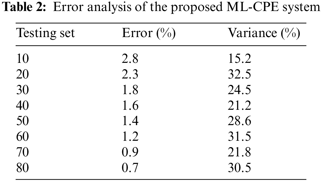
The error analysis of the proposed ML-CPE system’s training and the testing dataset is depicted in Figs. 9 and 10. The simulation analysis is done by varying the training and testing dataset. The respective simulation outcomes of the proposed ML-CPE system in terms of error and variance are evaluated. The proposed ML-CPE system with a machine learning model enhances system performance in training and testing conditions. The training dataset requires more time to train the system, and the testing dataset produces higher simulation results with higher accuracy. The proposed ML-CPE system is designed in this section, and the findings of the system are shown. The simulation outcomes such as error, variance, power, the accuracy of the proposed ML-CPE system, and the results are compared with the existing models. The proposed ML-CPE system with a machine learning model exhibits higher system performance.

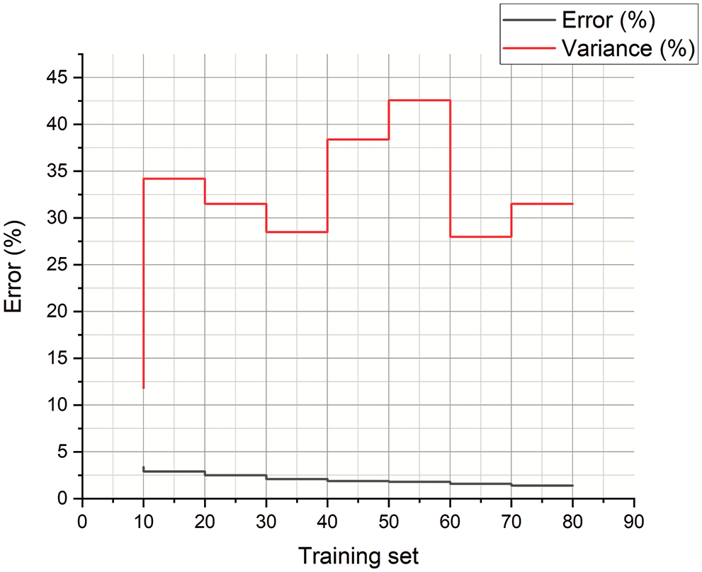
Figure 9: Error analysis of the training dataset

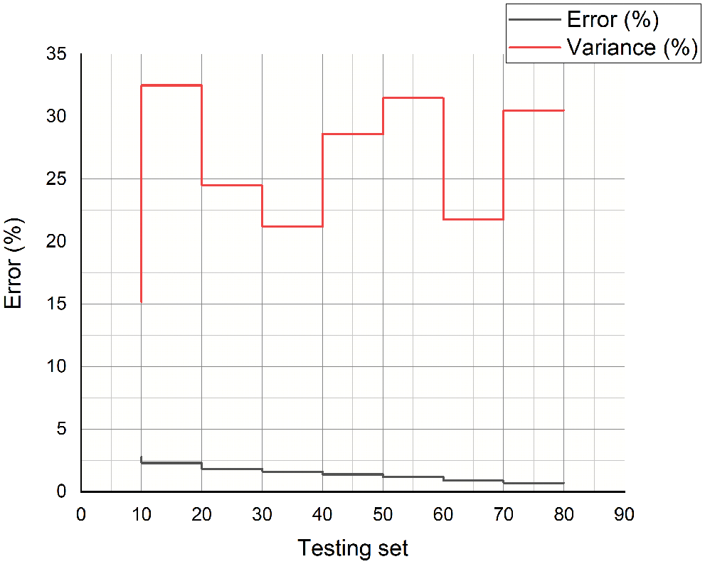
Figure 10: Error analysis of the testing dataset

5  Conclusion and Future Scope

Due to actual time and resources restrictions, it is impossible to do the methodology for all experiments. That is not able to precisely verify the entire sample data on complicated circuits. It advocated using advanced analytics to anticipate and not verify the proposed method consists of a training set. A model is being trained by the thorough analysis outcomes of a few experiments. The algorithm is used to forecast the power requirements of the other techniques to identify any hazardous power testing. The technique is shown to forecast the testing power requirements for most examinations effectively. Because it uses precise simulation figures from a few tests, the inaccuracy would be less than 6%. The findings from experiments demonstrate that predictive approaches reduce hours of running time to milliseconds for proper research. The machine learning method in aspects of runtime and failure rates was determined to be the finest. Overall, a machine learning forecast has been proven to be an excellent substitute for the correct reproduction of all training set to discover essential assessments of energy when they can’t be carried out. More criteria such as time-related characteristics are examined in the future study more to reduce errors.

Acknowledgement: This work supported by Dr S Karthik, SRM Institute of Science and Technology. We would also like thank to SRM Institute of Science and Technology, Vadapalani Campus, Chennai, Tamilnadu, India.

Funding Statement: The authors received no specific funding for this study.

Conflicts of Interest: The authors declare that they have no conflicts of interest to report regarding the present study.

References

1. D. Öhlinger, J. Maier, M. Függer and U. Schmid, “The involution tool for accurate digital timing and power analysis,” Integration, vol. 76, pp. 87–98, 2021. [Google Scholar]
2. X. Cai, R. Li, S. Kuang and J. Tan, “An energy trace compression method for differential power analysis attack,” IEEE Access, vol. 8, pp. 89084–89092, 2020. [Google Scholar]
3. D. Utyamishev and I. Partin-Vaisband, “Real-time detection of power analysis attacks by machine learning of power supply variations on-chip,” IEEE Transactions on Computer-Aided Design of Integrated Circuits and Systems, vol. 39, no. 1, pp. 45–55, 2020. [Google Scholar]
4. F. Kenarangi and I. Partin-Vaisband, “Exploiting machine learning against on-chip power analysis attacks: Tradeoffs and design considerations,” IEEE Transactions on Circuits and Systems I: Regular Papers, vol. 66, no. 2, pp. 769–781, 2019. [Google Scholar]
5. M. A. Xiangliang, L. I. Bing, W. A. N. G. Hong, W. U. Di, Z. H. A. N. G. Lizhen et al., “Non-profiled deep-learning-based power analysis of the SM4 and DES algorithms,” Chinese Journal of Electronics, vol. 30, no. 3, pp. 500–507, 2021. [Google Scholar]
6. S. Syed, R. Thriveni and P. V. A. Khan, “A novel approach of low power, less area, and economic integrated circuits,” Soft Computing and Signal Processing, vol. 898, pp. 471–483, 2019. [Google Scholar]
7. S. R. Shanmugham and S. Paramasivam, “Survey on power analysis attacks and its impact on intelligent sensor networks,” IET Wireless Sensor Systems, vol. 8, no. 6, pp. 295–304, 2018. [Google Scholar]
8. C. Luo, Y. Fei, L. Zhang, A. A. Ding, P. Luo et al., “Power analysis attack of an AES GPU implementation,” Journal of Hardware and Systems Security, vol. 2, no. 1, pp. 69–82, 2018. [Google Scholar]
9. S. Vennapusapalli, G. M. Sreerama-Reddy and R. R. Patel, “Analysis of coupling transition for the encoded data and its logical level power analysis,” Data Engineering and Communication Technology, vol. 63, pp. 183–192, 2021. [Google Scholar]
10. R. Agrawal, R. Vemuri and M. Borowczak, “A state machine encoding methodology against power analysis attacks,” Journal of Electronic Testing, vol. 35, no. 5, pp. 621–639, 2019. [Google Scholar]
11. Z. Zhang, J. Dofe and Q. Yu, “Improving power analysis attack resistance using intrinsic noise in 3D ICs,” Integration, vol. 73, pp. 30–42, 2020. [Google Scholar]
12. S. R. Shanmugham and S. Paramasivam, “Power analysis attack resilient block cipher implementation based on 1-of-4 data encoding,” ETRI Journal, vol. 43, no. 4, pp. 746–757, 2021. [Google Scholar]
13. M. Masoumi, “Novel hybrid cmos/memristor implementation of the AES algorithm robust against differential power analysis attack,” IEEE Transactions on Circuits and Systems II: Express Briefs, vol. 67, no. 7, pp. 1314–1318, 2019. [Google Scholar]
14. H. Abbassi, F. Khalid, O. Hasan and A. M. Kamboh, “McSeVIC: A model checking based framework for security vulnerability analysis of integrated circuits,” IEEE Access, vol. 6, pp. 32240–32257, 2018. [Google Scholar]
15. T. Pathade, Y. Agrawal, R. Parekh and M. G. Kumar, “Structure fortification of mixed CNT bundle interconnects for nano integrated circuits using constraint-based particle swarm optimization,” IEEE Transactions on Nanotechnology, vol. 20, pp. 194–204, 2021. [Google Scholar]
16. K. Palma and F. Moll, “Analysis of random body bias application in FDSOI cryptosystems as a countermeasure to leakage-based power analysis attacks,” IEEE Access, vol. 9, pp. 114977–114988, 2021. [Google Scholar]
17. A. K. Khana, H. J. Mahantab and A. Chakraborty, “Investigating the blinding approach to resist power analysis attacks on modular exponentiation,” International Journal of Computational Intelligence & IoT, vol. 1, no. 1, pp. 58–63, 2018. [Google Scholar]
18. P. Ashok and K. B. Vettuvanam-Somasundaram, “Charge balancing symmetric pre-resolve adiabatic logic against power analysis attacks,” IET Information Security, vol. 13, no. 6, pp. 692–702, 2019. [Google Scholar]
19. D. Jayasinghe, A. Ignjatovic, R. Ragel, J. A. Ambrose and S. Parameswaran, “QuadSeal: Quadruple balancing to mitigate power analysis attacks with variability effects and electromagnetic fault injection attacks,” ACM Transactions on Design Automation of Electronic Systems (TODAES), vol. 26, no. 5, pp. 1–36, 2021. [Google Scholar]
20. Y. Wen and W. Yu, “Breaking LPA-resistant cryptographic circuits with principal component analysis,” Integration, vol. 80, pp. 1–4, 2021. [Google Scholar]
21. S. Fahd, M. Afzal, H. Abbas, W. Iqbal and S. Waheed, “Correlation power analysis of modes of encryption in AES and its countermeasures,” Future Generation Computer Systems, vol. 83, pp. 496–509, 2018. [Google Scholar]
22. V. Shavali, G. M. Sreerama-Reddy and P. Ramana-Reddy, “Reduction of coupling transition by using multiple encoding technique in data bus and its power analysis,” in Innovations in Electronics and Communication Engineering, Singapore: Springer, pp. 345–353, 2019. [Google Scholar]
23. D. Thompson and H. Wang, “Integrated power signature generation circuit for IoT abnormality detection,” ACM Journal on Emerging Technologies in Computing Systems (JETC), vol. 18, no. 1, pp. 1–13, 2021. [Google Scholar]
24. H. Sun and R. Grishman, “Employing lexicalized dependency paths for active learning of relation extraction,” Intelligent Automation & Soft Computing, vol. 34, no. 3, pp. 1415–1423, 2022. [Google Scholar]
Cite This Article
Copyright © 2023 The Author(s). Published by Tech Science Press.
This work is licensed under a Creative Commons Attribution 4.0 International License , which permits unrestricted use, distribution, and reproduction in any medium, provided the original work is properly cited.
Downloads
Citation Tools