Classification of Brain Tumors Using Hybrid Feature Extraction Based on Modified Deep Learning Techniques

1  Introduction

Cancer is the leading cause of mortality worldwide, as around ten million patients died in 2020 [1,2]. Cancer, a term that encompasses any presence of one or many tumors, refers to the uncontrollable growth of cells inside the human body. This growth can be slow or aggressive [2–5]. This phenomenon occurs suddenly at any age without any noticeable symptoms [5,6]. This deadly disease requires early detection and diagnosis to increase survival rates. In many situations, cancer is fatal if no suitable treatment is provided [6,7]. The World Health Organization (WHO) reported that around 80,000 cases of BrT are discovered in the United States (US) yearly [1,2]. Among these cases, 32%–34% are considered very aggressive or malignant [1]. Physicians and radiologists have discovered more than 120 types of brain cancers, which are differentiated according to their locations or types of cells involved [7–9].

Brain cancer detection has been studied for over a decade using various imaging techniques, such as CT scans and MRIs. Multiple studies have been performed to improve brain tumor diagnoses using different technologies [2,4–10]. These technologies aim to save lives, improve patients’ quality of life, or reduce the need for surgery. Effective cancer treatments include chemotherapy, radiation, and surgery [1,4,7–12].

Particular attention to the process of diagnosing brain tumors is critical to reducing mortality rates [13,14]. Brain tumor diagnosis at an early stage of the disease requires the involvement of different imaging modalities [12,13]. Regardless of the imaging modality, image segmentation is a necessary step in analyzing scans of the brain. The segmentation process is critical to the accuracy of diagnoses since any error in imaging leads to undesired findings. In healthcare facilities, physicians rely on radiologists to provide accurate results from their segmentation procedures. These procedures are performed manually by radiologists, which can lead to errors due to human error or misanalysis [15–20]. Manual segmentation is time-consuming and requires expertise and knowledge, especially when dealing with sensitive organs such as the brain [21,22]. A reliable, dependable, and trustworthy automated system for image segmentation can be very helpful [18,21–25].

Nowadays, deep-learning techniques are involved in various fields, such as education, industry, and medicine, due to their highly accurate results in Computer Vision (CV). With improvements in Artificial Intelligence (AI), the use of deep-learning tools has significantly improved in its utility, especially in the healthcare domain [25,26].

1.1 Research Problem

Various AI-driven models have been developed to perform automated segmentation to attain high accuracy for cancer segmentation already. Specifically, deep-learning techniques (DLs), such as VGG-19 and LSTMs, can be efficiently utilized in different applications to perform segmentation. These methods require no human intervention to extract requisite mandatory characteristics to complete the segmentation process of diagnosis [1,3,6]. Automatic segmentation and diagnosis of brain cancer using deep-learning techniques can save lives and prevent further tumor growth. Numerous approaches, such as those in [1–6], were implemented to segment brain tumors using medical images, such as CT scans and MRIs. Nevertheless, various developed models provided an average accuracy between 90% and 98%. The challenge that this study takes on is integrating VGG-19 and LSTMs in a single, reliable, and efficient system. This article proposes a middleware framework that integrates VGG-19 and LSTMs, to perform the segmentation and categorization procedures of brain tumor diagnosis. These two DLs segment the medical images and classify the discovered masses as either slow-grow or aggressive. Slow-grow represents noncancerous tumors, known as benign, and aggressive denotes the cancerous masses, known as malignant.

1.2 Research Motivations and Contributions

The motivations of this study are summarized as follows:

•   To develop efficient and effective diagnostic procedures.

•   To enhance the accuracy of tumor classification using DL algorithms.

•   To reduce the time and expertise required to accurately diagnose and classify brain tumors.

•   To improve an oncologist’s ability to treat patients with brain cancer quickly and effectively.

This study aims to implement a middleware that integrates VGG-19 and LSTMs to act as a complete system for the segmentation and classification of BrT. Contributions to the literature include:

a)   Developing a complete BrT diagnosis-based model using MRIs from five datasets.

b)   Implementing a middleware framework that integrates two DLs to extract the necessary features for the classification part.

c)   Using an analysis of the performance of the presented model based on its efficacy on five publicly available datasets from Kaggle. The analysis will measure the accuracy, dice, precision, specificity, and F-score.

This article is organized as follows: Section 2 details the related work, and Section 3 completely explains the presented system. Section 4 contains details of the conducted experiments to evaluate the system, and Section 4 offers a discussion of the results. The conclusions are presented in Section 5.

2  Literature Review

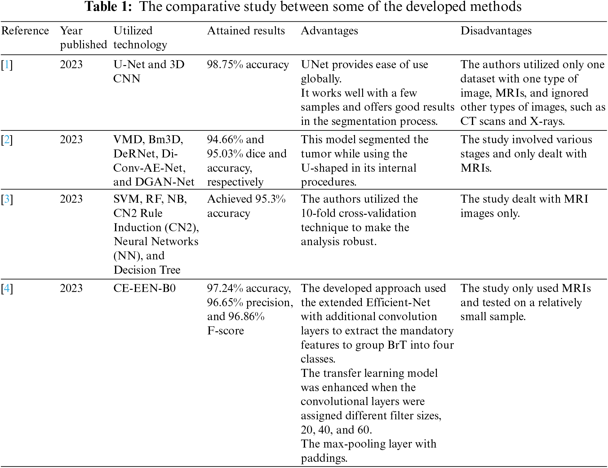
The authors in [1] developed a combinative UNet and 3D CNN model to segment BrT. Two models were used to segment images of tumors. The models achieved an accuracy average of 98.75%. In the first stage, Gray Level Co-occurrence (GLC) and Vantage Point Tree (VPT) tools extracted the needed features from MRI images. A classifier was involved in performing the final classification process. The GLC tool was used to find the brightness differences between pixels and store these differences in a matrix. At the same time, VPT was utilized to locate centers of the deployed data to separate data recursively. The authors rescaled all inputs with a fixed size of 128 × 128. Different chunks of data from one to ten were used to compare the developed model with other implemented algorithms in terms of accuracy, precision, specificity, sensitivity, and F-score. The authors in [1] focused their analysis on precision and obtained almost 98.69% precision for whole chunks of data. For comparison, the proposed system utilized five datasets to evaluate its model using different performance quantities. When two activation functions were used, namely Rectified Linear Unit (ReLU) and Leaky ReLU, this system achieved 97.32% and 98.265% for dice and accuracy. Moreover, other quantities reached values between 98.43% and 99.32%. These findings indicate that the presented system yields better results than the developed algorithm in [1].

In [2], El-Henawy et al. developed a framework to segment 3D MRIs of BrT using various tools to remove Rician and Speckle noise. The authors used Vibrational Mode Decomposition (VMD), Block-matching and 3D filtering (Bm3D), the Deep Residual Network (DeRNet), the Dilated Convolution Auto-encoder Denoising Network (Di-Conv-AE-Net), and the Denoising Generative Adversarial Network (DGAN-Net) and achieved 94.66% and 95.03% dice and accuracy, respectively. The presented system uses two DL techniques that act together as one complete tool to extract 28 features from inputs. The simpler technique reached 97.32% and 98.265% dice and accuracy. In addition, five datasets were used to train, validate, and test this model. Moreover, this model has an added feature: it segments the detected masses of tumors in two colors, where each color denotes a utilized activation function.

Asiri et al. in [3] provided a profound analysis of six Machine Learning (ML) algorithms on a utilized dataset from Kaggle to categorize BrT. The authors considered accuracy, the area under the Receiver Operating Characteristic (ROC) curve, precision, sensitivity, and F-score in their analysis. The six algorithms used were Support Vector Machine (SVM), Random Forest (RF), Naïve Bayes (NB), CN2 Rule Induction, Neural Networks (NN), and Decision Tree. The most effective algorithm was SVM, which achieved 95.3% accuracy in categorizing tumors as they appeared on MRIs. The proposed system in this research conducts an intensive analysis of a different set of unique characteristics to not only classify but segment BrT. The model is deployed on five datasets, as stated earlier. Two DLs are incorporated using the dedicated middleware framework and two activation functions. Improving upon [3], 98.265% accuracy was achieved. The obtained outcomes imply that the proposed method outstands all mentioned ML algorithms in [3] in accuracy.

In a study quite similar to this one, Mahesh et al. in [4] developed a model to detect and classify BrT. Their study classified according to a tumor’s location, identified using an extended Deep Convolutional Neural Network (DCNN) tool with feed-forward mode on MRIs. This tool was Contour Extraction-based Extended EfficientNet-B0 (CE-EEN-B0). It had three convolutional layers, one max-pooling layer, and one global average pooling layer. Four groups of BrT were classified with 97.24%, 96.65%, and 96.86% accuracy, precision, and F-score, respectively. A dataset of 3,264 MRIs was used. The authors used the ReLU activation function in their approach. Four performance quantities were used to evaluate the model: recall, accuracy, F-score, and precision. In contrast, this study utilizes five datasets and six performance metrics to evaluate its model: dice, accuracy, F-score, sensitivity, precision, and specificity. The presented algorithm achieved 98.265%, 97.32%, 98.77%, 98.46%, 98.69%, and 99.24% accuracy, dice, sensitivity, precision, specificity, and F-score, respectively. These values show that the presented model surpasses the developed method in [4] in all considered measurements of success.

Table 1 compares some of the developed approaches in the literature in terms of the utilized technology, obtained findings, advantages, and disadvantages.

3  The Proposed Algorithm

3.1 Problem Statement

Recently, researchers have turned their focus to utilizing deep-learning technologies in the medical field due to their significant achievements regarding accuracy. Distinguishing slow-grow or aggressive tumors inside the brain using MRI or CT scan images has especially recently achieved remarkable attention due to increased mortality rates related to BrT. Manually analyzing the necessary extracted characteristics to discover and classify BrT masses is time-consuming and requires expert high skills. Thus, building a completely automated system to segment images, identify BrT, and perform the categorization of tumors as slow-grow or aggressive processes is crucial. Recently, researchers have turned their focus to utilizing deep-learning technologies in the medical field due to their significant achievements regarding accuracy. This study proposes a practical middleware framework to integrate VGG-19 and LSTMs and create a single model that efficiently and accurately extracts features from multiple imaging modes to diagnose and classify cancers.

3.2 Deep-Learning Tools (DLTs)

3.2.1 VGG-19

VGG-19 accepts any input sized 224 × 224 × 3. It is another version of the Convolutional Neural Network (CNN) and has fourteen convolutional layers, three fully connected (FC) layers, and five max-pooling layers, as depicted in Fig. 1. Each convolutional layer is 3 × 3, and every max-pooling size is 2 × 2.

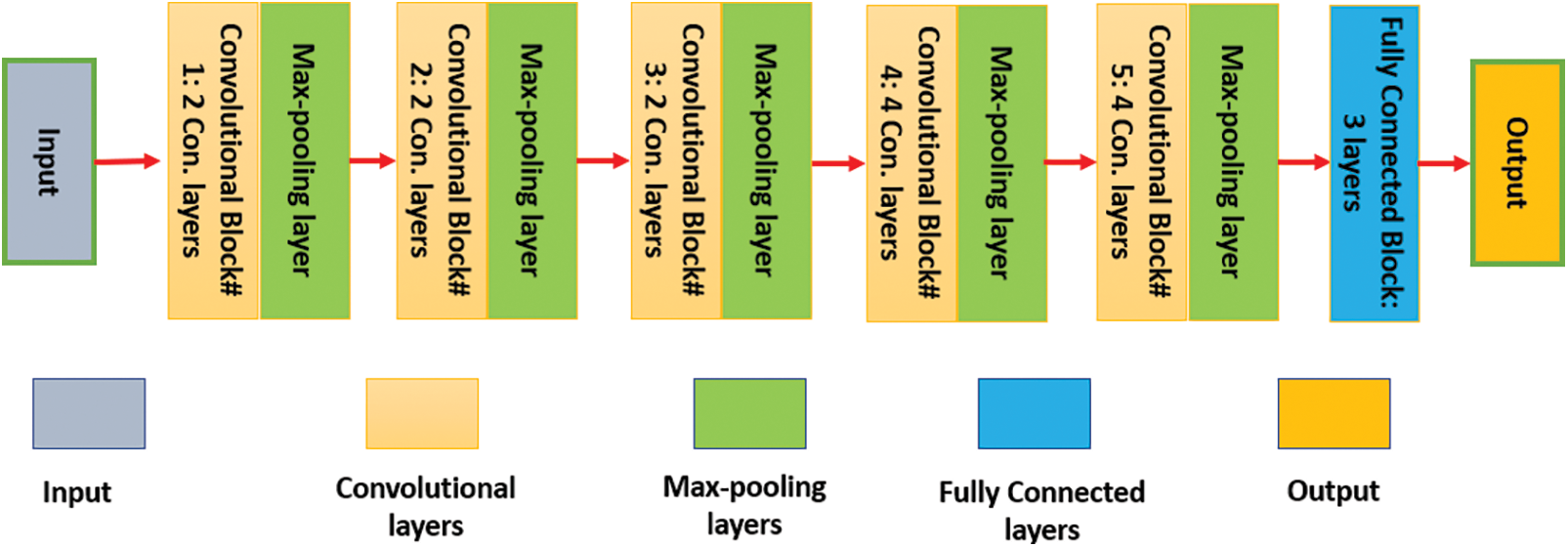
Figure 1: The internal structure of the VGG-19 network

Each convolutional layer results from multiplication between an input Ai and a bank inside a filter Bi [27]. The output of any convolutional layer Ci is computed using Eq. (1) as follows:

Cij=∑ij(Ai∗Bi)+Ri(1)

Ri represents the regularization bias term. For nonlinear cases, the convolutional layer is calculated using the ReLU activation function as in Eq. (2) [27]:

Ci=Max (0,Ai)(2)

3.2.2 LSTMs

LSTMs are a type of Recurrent Neural Network (RNN) [28]. This network comprises various units. Each unit contains four main parts: three gates and a cell state. These three gates are the input, forget, and output [28]. Tanh is the activation function utilized in this network. Fig. 2 illustrates an internal structure of any LSTM unit.

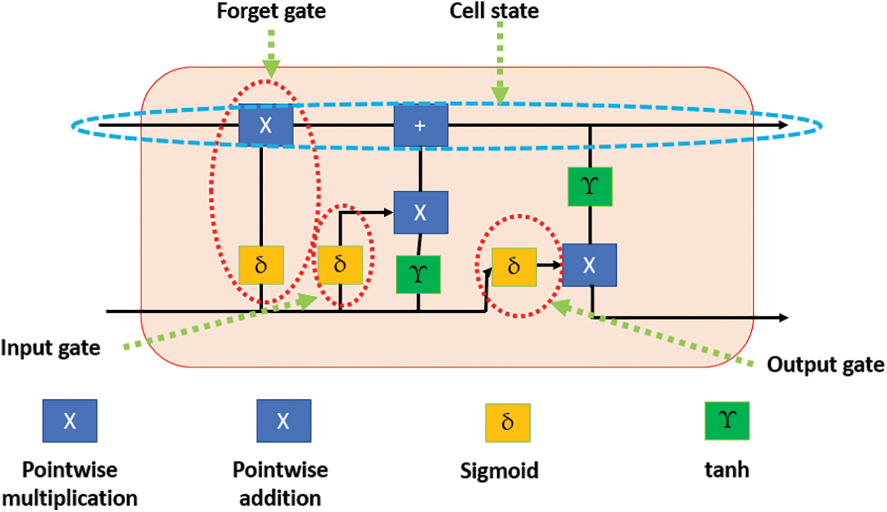
Figure 2: The block diagram of the LSTM unit

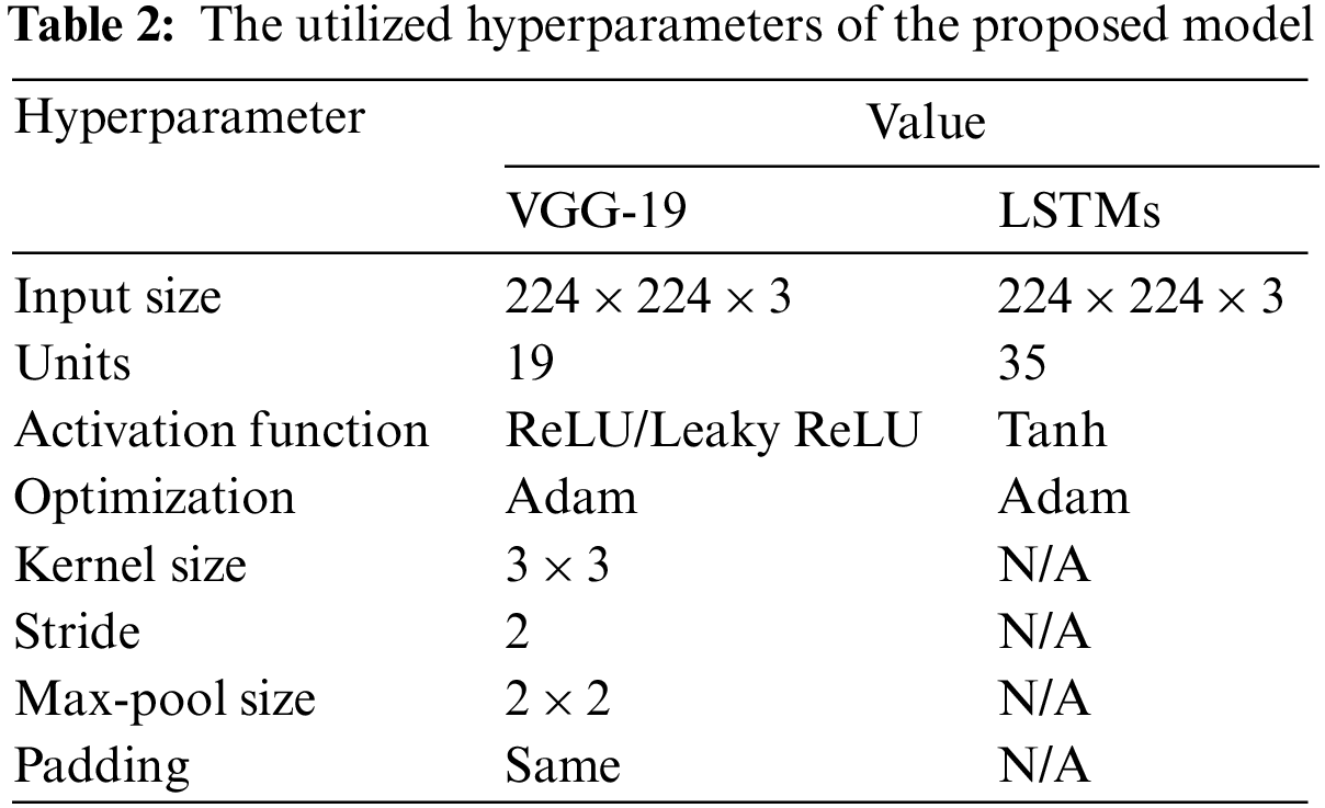
Table 2 shows all the hyperparameters used for this network in the presented system.

For the sigmoid function, the output of each gate is computed as shown in Eq. (3):

It=wiAt+Uiht−1+Ri

Ft=wfAt+Ufht−1+Rf(3)

Ot=woAt+Uoht−1+Ro

where t refers to an instance time, I represents the input, F represents the forget, O represents the output, w denotes the weights in each gate, U is a recurrent connect, and h represents the hidden layer. The weights matrix is computed as in Eqs. (4) to (6):

Wij(t+1)=wij(t)+L(t)h(t)(Ai–wij(t))(4)

h(t)=exp⁡(d2ij/(2∗rad2(t)))(5)

rad(t+1)= RND [(rad(t)−1)∗(1–t/T)]+1(6)

L(t) denotes the learning rate, which is 0.01 for the ReLU and 0.0001 for Leaky ReLU. The value dij represents the distance between every two consecutive neurons in the network, rad refers to the radius of the neighbor neuron, T refers to the frequency of learning, and RND denotes the rounding function. The output from each unit is calculated using the Leaky ReLU activation function as depicted in Eq. (7):

Ci=Max(∂Ai,Ai)(7)

∂ takes a small value; this value varies between 0.01 to 0.2.

3.3 Datasets

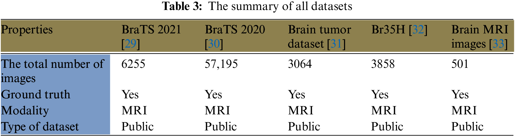
Five large datasets from Kaggle are utilized in this study to train the model. The first dataset (BraTS 2021) from [29] is 12.4 GB and contains 6,255 MRI images. This dataset includes four classes: 1) T1; 2) T1Gd; 3) T2-weighted (T2); and 4) T2-FLAIR. Neuroradiologists with significant experience approved these images. The second dataset (BRaTS 2020) from [30] is 7 GB with 57,195 MRI images. It contains the same four classes as the first dataset. The third dataset from [31] is approximately 900 MB and comprises 3,064 T1-weighted contrast-enhanced images from 233 participants. It includes three kinds of BrT: meningioma (708 images), glioma (1426 images), and pituitary tumors (930 images). The fourth dataset from [32] contains 3,858 MRI images with a size of 88 MB. The fifth dataset from [33] has 501 MRI images and is nearly 16 MB. These datasets are divided into two classes: one is dedicated to training the model and represents 70% of the images, while the other is involved in the validation and testing processes. The second group is designated as follows: 10% for validation and 20% for testing. Table 3 lists a summary of all utilized datasets in this study, listing the total number of images, ground truth, modality, and dataset type. In this research, the number of assigned images for training, validation, and testing sets was 496,107,089, and 14,174, respectively.

3.4 The Proposed Methodology

This study proposes a complete system for BrT diagnosis using two DL techniques, VGG-19, and LSTMs. This system is an ensemble of two tools because, in combination, they offer significant improvements in feature extraction to other models and accurate, efficient performance. DL technique extracts 14 unique characteristics and merges them in the middleware framework that is implemented for this purpose. This framework makes both DL tools work as one; thus, in total, 28 unique features are extracted, including radius, texture, area, compactness, smoothness, and perimeter after the inputs are segmented. In total, the proposed system extracts 1,984,444 unique features from all utilized datasets. These characteristics assist the presented model in categorizing the detected masses into three classes. These classes are called healthy, slow-grow, and aggressive. A clustering algorithm is required for the system to cluster the potentially detected mass tumors into their suitable groups, namely the self-organization map. As stated earlier, the main objective of using this clustering algorithm is to map the data to relevant groups. This clustering approach works based on two procedures; the first procedure is to normalize a weight vector of each neuron using a current input vector x and its corresponding neuron value. The second procedure is to select a neuron node according to a minimum result of the Euclidian distance between the neuron value and the weight. Then, the weight matrix is modified regularly, as depicted in Eqs. (4) to (6). Fig. 3 shows an architecture of the self-organization map structure.

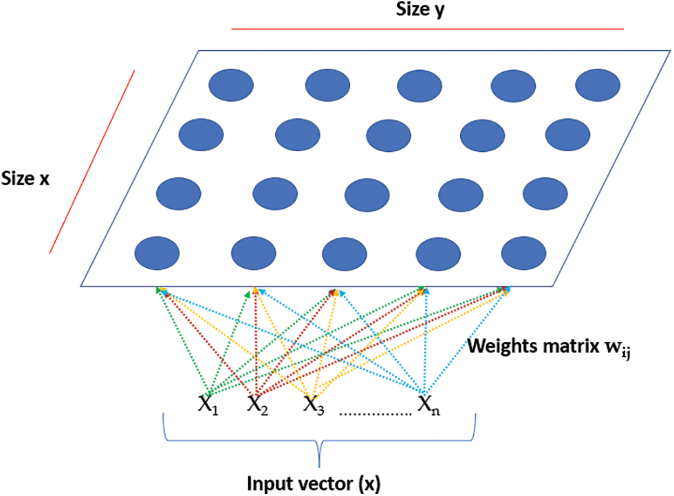
Figure 3: The architecture of the self-organization map structure

The VGG-19 tool is comprised of 14 convolutional layers and five max-pooling layers, as depicted in Fig. 1. The LSTMs technique contains 35 units. The proposed system consists of three stages, as illustrated in Fig. 4. Stage 1 is the image preprocessing stage; Stage 2 is the learning and feature extraction stage, and Stage 3 is the final classification procedure. These three stages are illustrated from top to bottom in Fig. 4. Fig. 5 offers a block diagram of the implemented middleware framework.

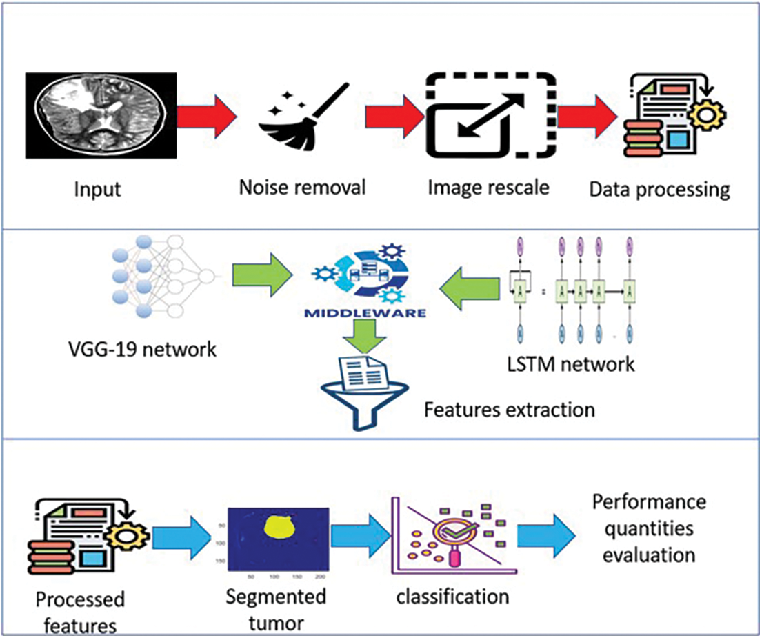
Figure 4: The architecture of the proposed system

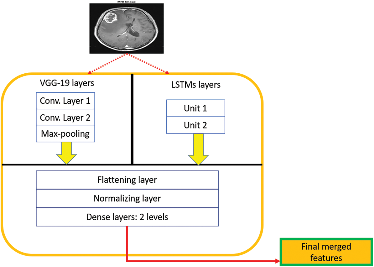
Figure 5: The architecture of the middleware framework

The middleware framework can be seen as a single structure with multi-layers, as depicted in Fig. 5. These multiple layers are stacked in a hierarchical form to extract the necessary characteristics from each DL tool efficiently. The utilized batch size in the middleware framework is 10. All extracted features are flattened and later normalized to avoid additional load on the system, reduce the processing time, and remove the overfitting problem. After that, the system classifies tumors as slow-grow or aggressive. For simplicity, “one” refers to the slow-grow type, “two” represents the aggressive type, and “three” denotes no cancer. Lastly, numerous performance quantities are evaluated including accuracy, dice, precision, sensitivity, specificity, and F-score. Additional details on the performance qualities are provided in the next section.

Inside the middleware framework, the input layers gather the preprocessed information from each DL technique and pass this data into the hidden layers from both models, which output the subsets of feature vectors. These vectors are reprocessed through the convolutional layers in a pipeline hierarchy. The final sets of feature vectors are flattened, normalized, and transformed into one dimension. The batch normalization layer is utilized to regulate the input of every layer. A final vector is generated in the last two dense layers, as depicted in Fig. 5.

The proposed system takes inputs from the five utilized datasets. Then, these inputs are preprocessed to clean them from noise, rescaled to the predefined size of the DL tools, converted into grayscale images, and the resultant pixels are transformed to floating points of decimal type. Then, the segmentation process begins and segments the detected masses from the rest of the image and outlines the tumors with a unique color. In this study, green is used to outline tumors using the ReLU activation function, and yellow is utilized to mark the outlined tumors using the Leaky ReLU activation function. Next, the DL techniques extract the necessary features. Each tool pulls 14 unique characteristics. The system is trained using both DL techniques on the provided datasets and categorizes the detected tumor masses into two classes, as stated earlier. The training dataset is composed of inputs with their labels, which the proposed model uses to learn intensively as time goes on. Accuracy is determined through the loss function, which shall be minimized.

Eq. (8) is used to obtain the desired outputs from the inputs.

C=f(A)(8)

C refers to the outputs, A denotes the inputs, and f represents the mapping function, which is the self-organization map algorithm. This algorithm is modified to produce a new outcome when applying a new input. Two learning rates, ℓ1 and ℓ2 are used, where ℓ1 is dedicated to the ReLU activation function and ℓ2 is assigned to the Leaky ReLU activation function. Both rates take values of 0.01 and 0.0001, respectively. The training lasted approximately 9 h. The following pseudo-codes depict how the suggested algorithm works:

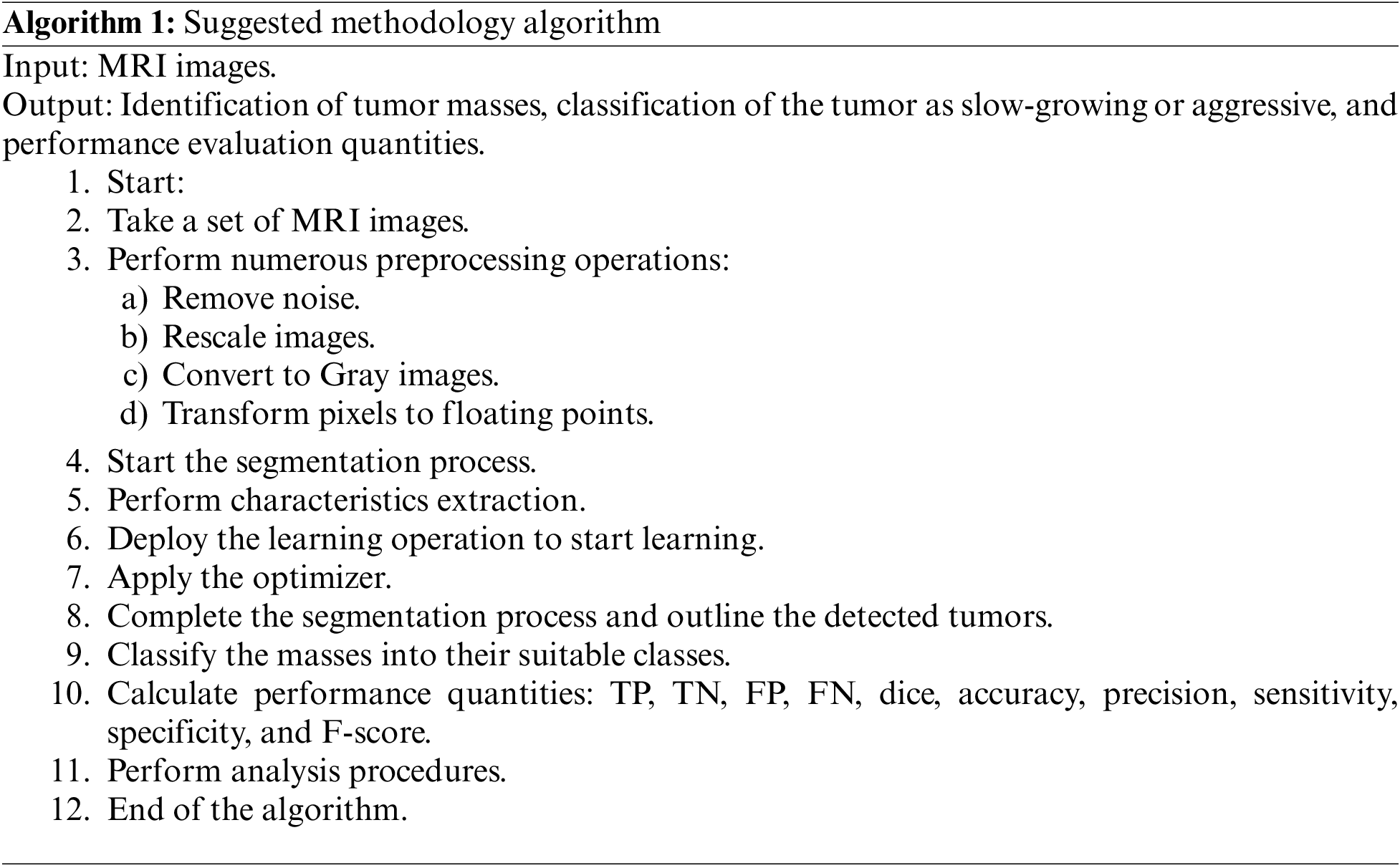
Various quantities are measured in the proposed model:

1.    True Positive (TP): an indicator of which the true class was properly detected and categorized.

2.    False Positive (FP): an indicator of how many true inputs was improperly categorized.

3.    True Negative (TN): it tells how the proposed system predicted the negative class accurately.

4.    False Negative (FN): this metric is an output of how many negative classes were detected wrongly.

Precision (Pre): is calculated as shown in Eq. (9):

Pre = TP/(TP+FP)(9)

Sensitivity (Sen): also known as recall, is calculated as in Eq. (10):

Sen = TP/(TP+FN)(10)

Accuracy (Acc): is computed with Eq. (11):

Acc =(TP+TN)/[TP+TN+FN+FP](11)

Specificity (Spe): this parameter is computed via Eq. (12):

Spe = TN/(TN+FP)(12)

F-score: this metric is determined via Eq. (13):

F−Score =2×[(Pre×Sen)/(Pre+Sen)](13)

Dice (Dic): denotes an overlap degree between the outcomes of the proposed system and the actual data. This quantity is determined as shown in Eq. (14):

Dic =2TP/(2TP+FP+FN)(14)

4  Results and Discussion

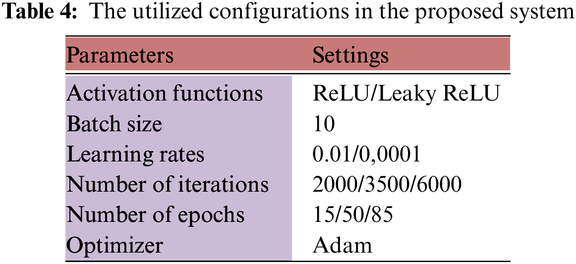
This section is dedicated to describing the experiment process and the achieved results. Numerous tests were conducted to evaluate the presented system and validate its efficiency. The performance was assessed using five public datasets from Kaggle. As mentioned, the evaluation process calculated six quantities to verify the proposed system’s functionality. The platform used was MATLAB R2017b. The training and testing data were divided 70:20, respectively. The system used Binary Cross Entropy (BCE) as its loss function. Table 4 lists the settings being used during the training and testing stages.

There were 49,610 total trained MRI images and 14,174 testing images as stated earlier. Various scenarios were evaluated and investigated to discern how the system is able to spot and categorize BrT.

MATLAB uses a variety of built-in functions and toolboxes to handle and operate various types of images. This platform was installed and run on a desktop machine that runs Windows 11 Pro, an Intel Core i7 8th generation chip with 2.0 GHz processing power and 16 GB of RAM. This study used quantitative and qualitative types of evaluation on the required performance quantities.

In the testing stage, all images were processed and then an average value was computed for each performance measurement. This operation lasted 273 min when the system ran 6,000 times. Table 5 lists the average percentage results of the considered quantities when two activation functions were deployed on the testing images over 3500 iterations.

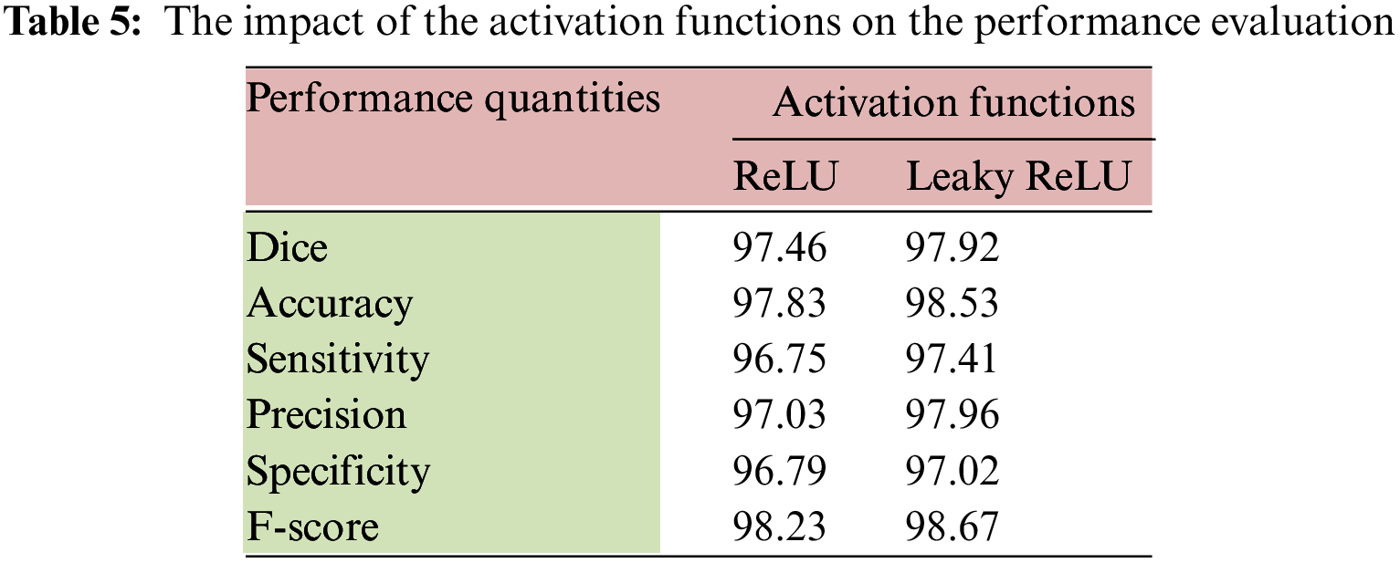
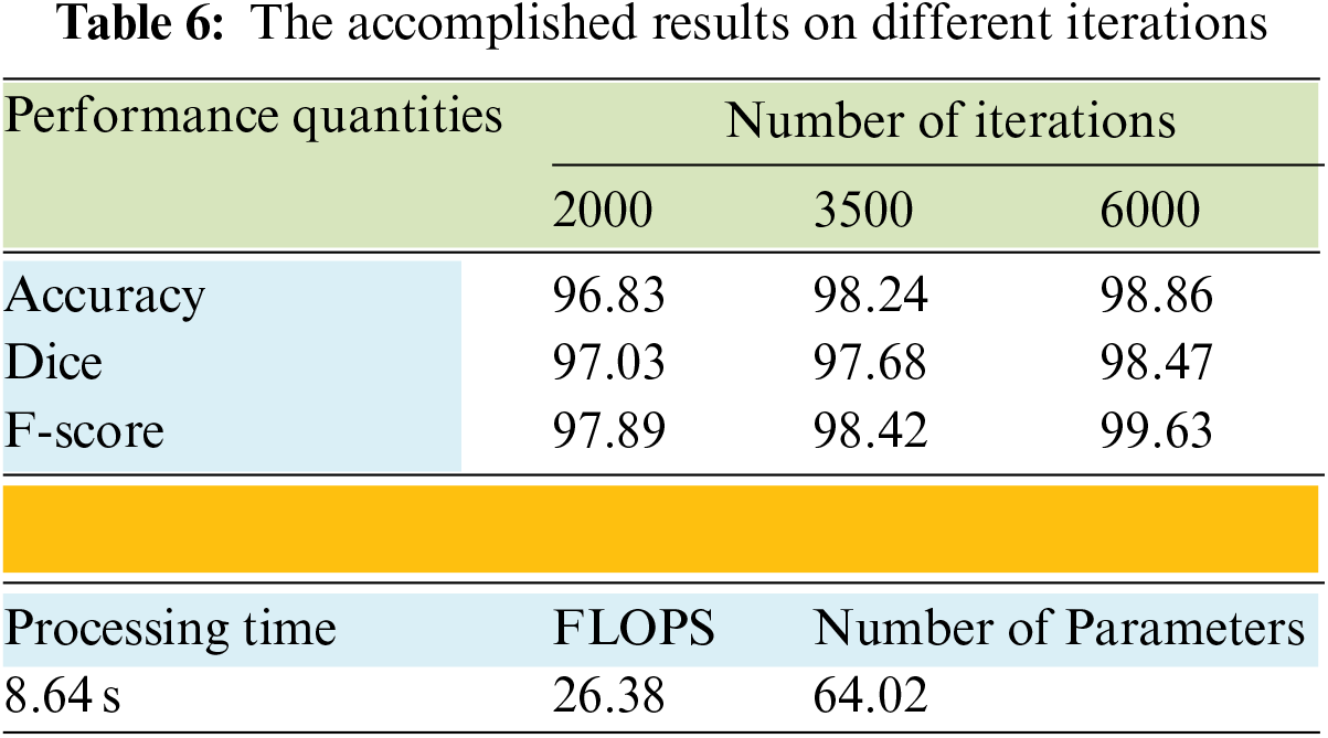
The performance of the model slightly improved when the Leaky ReLU function was applied. Table 5 shows that the highest accuracy was achieved with the second activation function. The dice improved by 0.472%, the accuracy enhanced by 0.716%, and F-score went up by 0.448%. Table 6 provides the results of the average achieved accuracy, dice, and F-score with different iteration numbers using the Leaky ReLU activation function. The quantities of every performance measure improved significantly when the number of iterations increased, as shown in Table 6. The processing time in seconds, the number of utilized parameters, and the Floating-Point Operation per Second (FLOPS) were also determined in this study. These quantities were computed using an input size of 224 × 224 × 3. These metrics represent the computation complexity of the proposed system, as shown in Table 6. Both FLOPS and the number of parameters were found to be in millions. The results indicate that the system is pervasive in computations and attains an above-average accuracy compared to other methods.

Figs. 6 and 7 illustrate samples of two inputs and their segmentation results in two colors. Once the ReLU function is applied, a tumor is denoted in yellow. A green mass denotes the output of the Leaky ReLU function.

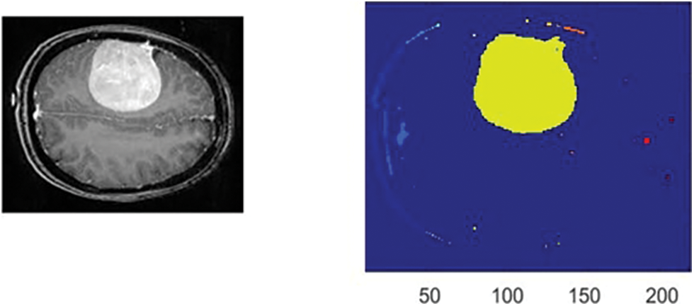
Figure 6: The obtained outcomes of the ReLU function

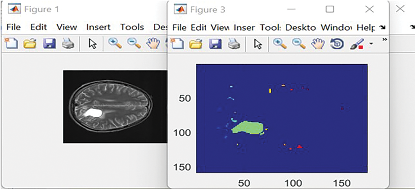
Figure 7: The obtained outcomes of the Leaky ReLU function

For the learning rate of 0.01, there were 465 total iterations and 15 epochs used. Each epoch had 31 iterations, and the system reached 99.8% accuracy. The accuracy curve steadied after five epochs, at which point the loss function also converged to almost zero. For the learning rate of 0.0001, the total number of iterations was 2,635, with 85 total epochs of 31 iterations each. The trained system achieved 98.4% accuracy. The presented algorithm became stable after 42 epochs.

Table 7 demonstrates the confusion matrix that was obtained by the presented system. Green refers to the properly discovered and identified types, while red represents improperly identified types.

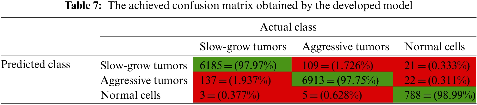
In Table 7, the suggested system categorized 6,185 slow-grow samples out of 6,315 resulting in 97.97% accuracy. For the aggressive type, it correctly classified 6,913 samples out of 7,072 offering 97.75% accuracy. For the third class, normal cells, the system categorized 788 samples out of 796 correctly. The total number of incorrectly classified samples was 297, which is relatively small compared to the set size, or 2.095% of all samples. This means approximately 98% of the set was accurately categorized.

The conducted comparative evaluation between the presented model and some implemented works from the literature is shown in Table 8. This evaluation includes the techniques used, dice, accuracy, and F-score. These outcomes reveal that the proposed model outperforms other methods in all considered quantities.

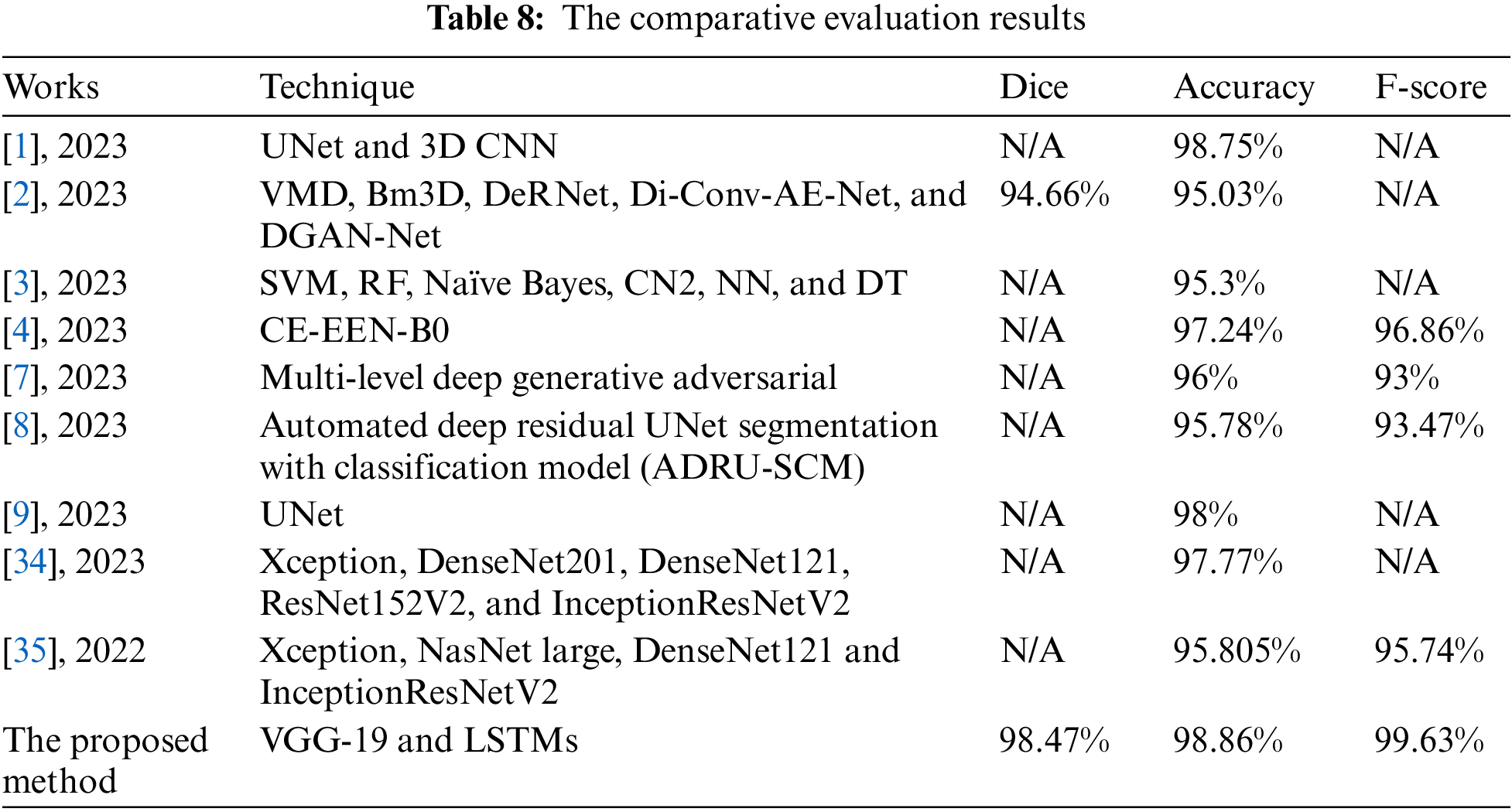
Fig. 8 illustrates a graphical representation of all achieved accuracy results in Table 8 except the work in [5].

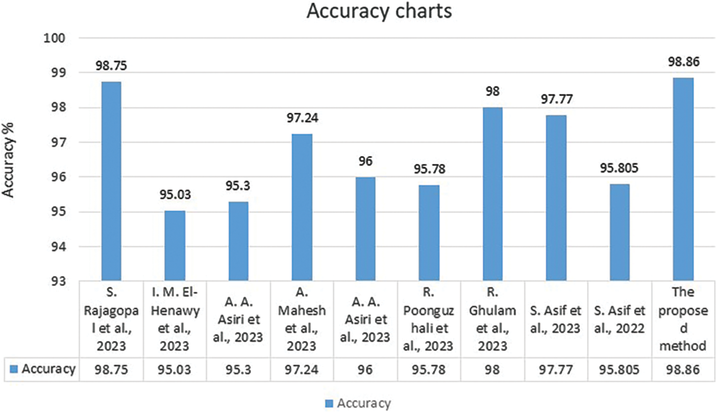
Figure 8: The comparative evaluation between the suggested algorithm and some related work [1–4,7–9,34,35] regarding the accuracy

The best achieved Mean Squared Error (MSE) when using the ReLU activation function was 0.0020283 occurred at epoch 24. When the Leaky ReLU activation function was deployed, the best MSE value was 0.0031075 and occurred at epoch 26. Fig. 9 displays the Receiver Operating Characteristic (ROC) curve that was obtained by the system using seven thresholds.

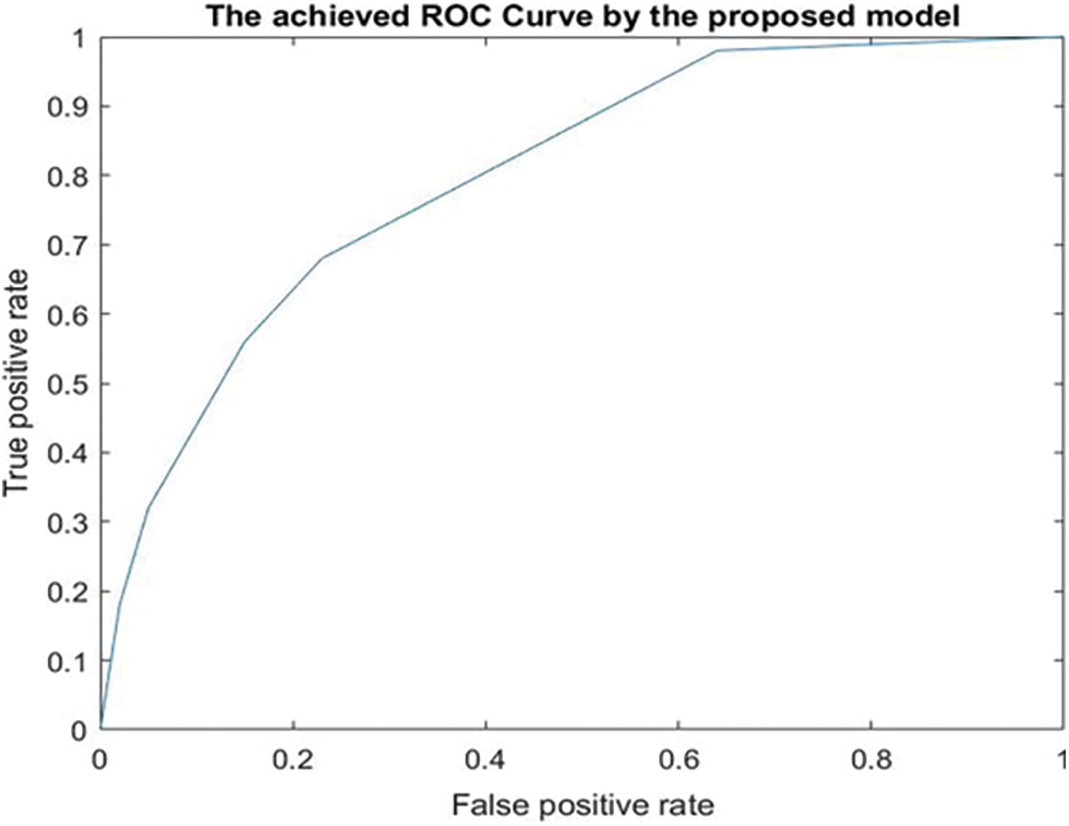
Figure 9: The achieved ROC curve

The conducted experiments and achieved results proved that the proposed algorithm can efficiently identify BrT masses and properly categorize them as slow-grow, aggressive, or healthy, as shown in Table 7. These classification results demonstrate that the system surpasses other methods in dice, accuracy, and F-score, as illustrated in Table 8. Regarding the dice metric, the developed method in [2] achieved the lowest value. The implemented algorithms in [2,3,6,8] attained the minimum accuracy results, whereas the models in [1,4,7,9] reached moderate values. Regarding the F-score quantity, the method in [7] achieved the minimum value, while the model in [4] achieved a moderate outcome. The suggested system obtained better results in terms of dice, accuracy, and F-score than any other study, as shown in Table 8. Table 5 displays the results of the system when two activation functions were applied. The Leaky ReLU function attained better results. The improvement is less than 1%, nevertheless, the slight improvement implies that the presented system can function adequately under different circumstances. Table 6 shows the obtained results of accuracy, dice, and F-score under a different number of iterations. These outcomes indicate that the system improved its findings significantly as the number of iterations increased. In addition, these values went higher when the number of iterations was 9000. However, this increment affects the performance of the execution time negatively. The execution time of every input was nearly 19.42 s.

The Leaky ReLU function took more execution time to reach the best value at Epoch 26. This was expected since the utilized learning rate for Leaky ReLU is smaller than the used rate in the ReLU function. The slower learning rate means that the system requires more time.

In this study, the implemented middleware framework was able to properly integrate two DL techniques: VGG-19, and LSTMs. These two techniques were incorporated with the self-organization map algorithm to achieve the best values for the mandatory features to complete the segmentation process and build up the classification procedures. The achieved outcomes are an indication for physicians and healthcare providers to inform them that the system can be widely deployed to assist them in diagnosing brain cancer early to provide suitable treatment plans.

5  Conclusion and Future Works

The presented system is fully automated and works very well to diagnose brain tumors, as shown in the obtained findings. These findings are exquisite and prove that this system has the capability to perform its functions precisely. As illustrated in the previous figures, this method involves two deep-learning techniques: ensembling and integrating VGG-19 and LSTMs through the middleware framework, which is implemented for this purpose. Along with the self-organization map algorithm, these DLs were able to diagnose the disease quickly, a result that indicates this method’s ability to detect cancer early, prepare minimally invasive treatment plans, and save lives.

In accordance with the utilized activation functions, this system can outline any detected masses in two colors. These tumors, if found, are categorized into two classes, and the system can tell where there is no mass, and the brain is healthy. Five different datasets from Kaggle were used to evaluate the suggested algorithm and it was found that the presented model surpasses all developed works in the literature on the most critical measurements. The achieved accuracy by this method ranges from 97.44% to 98.86%.

There is a limitation: the proposed system suffers from intensive computations. Luckily, this disadvantage can be overridden by using a machine with higher specifications than what was used in this study or by using a cloud-based system with high specifications and capabilities.

The authors intend to pursue further work to increase the accuracy, dice, and other performance quantities of their method using different types of images, such as CT scans, since this study uses only MRI images.

Acknowledgement: None.

Funding Statement: The authors received no funding.

Author Contributions: Study conception and design: T. Shawly and A. Alsheikhy; data collection: T. Shawly; analysis and interpretation of results: T. Shawly and A. Alsheikhy; draft manuscript preparation: T. Shawly. All authors reviewed the results and approved the final version of the manuscript.

Availability of Data and Materials: The utilized datasets in this research can be downloaded from the Kaggle website and their links are available from [29] to [33].

Conflicts of Interest: The authors declare that they have no conflicts of interest to report regarding the present study.

References

1. S. Rajagopal, T. Thanarajan, Y. Alotaibi and S. Alghamdi, “Biomedical brain tumor: Hybrid feature extraction based on UNet and 3DCNN,” Computer Systems Science and Engineering, vol. 45, no. 2, pp. 2093–2109, 2023. [Google Scholar]

2. I. M. El-Henawy, M. Elbaz, Z. H. Ali and N. Sakr, “Novel framework of segmentation 3D MRI of brain tumors,” Computer, Materials & Continua, vol. 74, no. 2, pp. 3490–3502, 2023. [Google Scholar]

3. A. A. Asiri, B. Khan, F. Muhammad, S. U. Rahman, H. A. Alshamrani et al., “Machine learning-based models for magnetic resonance imaging (MRI)-based brain tumor classification,” Intelligent Automation and Soft Computing, vol. 36, no. 1, pp. 299–312, 2023. [Google Scholar]

4. A. Mahesh, D. Banerjee, A. Saha, M. R. Prusty and A. Balasundaram, “CE-EEN-B0: Contour extraction based extended efficientnet-B0 for brain tumor classification using MRI images,” Computer, Materials & Continua, vol. 74, no. 3, pp. 5967–5982, 2023. [Google Scholar]

5. I. Mahmud, M. Mamun and A. Abdelgawad, “A deep analysis of brain tumor detection from MR images using deep learning networks,” Algorithms, vol. 16, no. 176, pp. 1–19, 2023. [Google Scholar]

6. H. Jain, G. Mainola, D. Rustagi, B. Gakhar and Gunjanchugh, “Brain tumor detection using image segmentation,” International Journal for Modern Trends in Science and Technology, vol. 8, no. 6, pp. 147–153, 2022. [Google Scholar]

7. A. A. Asiri, A. Shaf, T. Ali, M. Aamir, A. Usman et al., “Multi-level deep generative adversarial networks for brain tumor classification on magnetic resonance images,” Intelligent Automation and Soft Computing, vol. 36, no. 1, pp. 127–143, 2023. [Google Scholar]

8. K. R. Reddy and R. Dhuli, “A novel lightweight CNN architecture for the diagnosis of brain tumors using MR images,” Diagnostics, vol. 13, no. 312, pp. 1–21, 2023. [Google Scholar]

9. H. ZainEldin, A. A. Gamel, E. M. El-Kenawy, A. H. Alharbi, D. S. Khafaga et al., “Brain tumor detection and classification using deep learning and sine-cosine fitness grey wolf optimization,” Bioengineering, vol. 10, no. 18, pp. 1–19, 2023. [Google Scholar]

10. R. Asad, S. U. Rehman, A. Imran, J. Li, A. Almuhaimeed et al., “Computer-aided early melanoma brain-tumor detection using deep-learning approach,” Biomedicine, vol. 11, no. 1, pp. 1–22, 2023. [Google Scholar]

11. R. Zhang, S. Jia, M. J. Adamuand, W. Nie, Q. Li et al., “HMNet: Hierarchical multi-scale brain tumor segmentation network,” Journal of Clinical Medicine, vol. 12, no. 2, pp. 1–17, 2023. [Google Scholar]

12. A. A. Akinyelu, F. Zaccagna, J. T. Grist, M. Castelli and L. Rundo, “Brain tumor diagnosis using machine learning, convolutional neural networks, capsule neural networks and vision transformers, applied to MRI: A survey,” Journal of Imaging, vol. 8, no. 8, pp. 1–40, 2022. [Google Scholar]

13. A. Younis, L. Qiang, C. O. Nyatega, M. J. Adamu and H. B. Kawuwa, “Brain tumor analysis using deep learning and VGG-16 ensembling learning approaches,” Applied Sciences, vol. 12, no. 14, pp. 1–20, 2022. [Google Scholar]

14. S. Raghu and T. A. Lakshmi, “Brain tumor detection based on MRI image segmentation using U-Net,” Annals of the Romanian Society for Cell Biology, vol. 26, no. 1, pp. 579–594, 2022. [Google Scholar]

15. G. Latif, “Deep tumor: Framework for brain MR image classification, segmentation and tumor detection,” Diagnostics, vol. 12, no. 11, pp. 1–23, 2022. [Google Scholar]

16. N. A. Samee, N. F. Mahmoud, G. Atteia, H. A. Abdallah, M. Alabdulhafith et al., “Classification framework for medical diagnosis of brain tumor with an effective hybrid transfer learning model,” Diagnostics, vol. 12, no. 10, pp. 1–19, 2022. [Google Scholar]

17. G. T. Mgbejime, A. Hossin, G. U. Nneji, H. N. Monday and F. Ekong, “Parallelistic convolutional neural network approach for brain tumor diagnosis,” Diagnostics, vol. 12, no. 10, pp. 1–20, 2022. [Google Scholar]

18. C. D. Noia, J. T. Grist, F. Riemer, M. Lyasheva, M. Fabozzi et al., “Predicting survival in patients with brain tumors: Current state-of-the-art of AI methods applied to MRI,” Diagnostics, vol. 12, no. 9, pp. 1–16, 2022. [Google Scholar]

19. Y. E. Almalki, M. U. Ali, K. D. Kallu, M. Masud, A. Zafar et al., “Isolated convolutional-neural network-based deep feature extraction for brain tumor classification using shallow classifier,” Diagnostics, vol. 12, no. 8, pp. 1–12, 2022. [Google Scholar]

20. F. Ekong, Y. Yu, R. A. Patamia, X. Feng, Q. Tang et al., “Bayesian depth-wise convolutional neural network design for brain tumor MRI classification,” Diagnostics, vol. 12, no. 7, pp. 1–17, 2022. [Google Scholar]

21. D. T. Nguyen, S. H. Nam, G. Batchuluum, M. Owais and K. R. Park, “An ensemble classification method for brain tumor images using small training data,” Mathematics, vol. 10, no. 23, pp. 1–30, 2022. [Google Scholar]

22. S. Sharma, S. Gupta, D. Gupta, A. Juneja, H. Khatter et al., “Deep learning model for automatic classification and prediction of brain tumor,” Journal of Sensors, vol. 2022, 3065656, pp. 11, 2022. [Google Scholar]

23. M. Sharma, P. Sharma, R. Mittal and K. Gupta, “Brain tumour detection using machine learning,” Journal of Electronics and Informatics, vol. 3, no. 4, pp. 298–308, 2021. [Google Scholar]

24. N. Sravanthi, N. Swetha, P. R. Devi, S. Rachana, S. Gothane et al., “Brain tumor detection using image processing,” International Journal of Scientific Research in Computer Science, Engineering and Information Technology, vol. 7, no. 3, pp. 348–352, 2021. [Google Scholar]

25. N. Goyal and B. Sharma, “Image processing techniques for brain tumor identification,” in 1st Int. Conf. on Computational Research and Data Analytics (ICCRDA 2020), Rajpura, India, vol. 1022, pp. 012011, 2021. [Google Scholar]

26. N. Rani and S. Vashisth, “Brain tumor detection and classification with feed forward back-prop neural network,” International Journal of Computer Applications, vol. 146, no. 12, pp. 1–6, 2016. [Google Scholar]

27. Y. Said, A. Alsheikhy, T. Shawly and H. Lahza, “Medical images segmentation for lung cancer diagnosis based on deep learning architectures,” Diagnostics, vol. 13, no. 3, pp. 1–15, 2023. [Google Scholar]

28. E. M. Al-Ali, Y. Hajji, Y. Said, M. Hleili, A. Alanzi et al., “Solar energy production forecasting based on a hybrid CNN-LSTM-transformer model,” Mathematics, vol. 11, no. 3, pp. 1–19, 2023. [Google Scholar]

29. D. Schettler, 2021. [Online]. Available: https://www.kaggle.com/datasets/dschettler8845/brats-2021-task1 [Google Scholar]

30. Awsaf, 2020. [Online]. Available: https://www.kaggle.com/datasets/awsaf49/brats2020-training-data [Google Scholar]

31. J. Cheng, “Brain Tumor Dataset,” Figshare: Dataset, 2017. [Online]. Available: https://doi.org/10.6084/m9.figshare.1512427.v5 [Google Scholar] [CrossRef]

32. N. Chakrabarty, 2019. [Online]. Available: https://www.kaggle.com/datasets/navoneel/brain-mri-images-for-brain-tumor-detection [Google Scholar]

33. A. Hamada, 2022. [Online]. Available: https://www.kaggle.com/datasets/ahmedhamada0/brain-tumor-detection [Google Scholar]

34. S. Asif, M. Zhao, F. Tang and Y. Zhu, “An enhanced deep learning method for multi-class brain tumor classification using deep transfer learning,” Multimedia Tools and Applications, vol. 82, pp. 31709–31736, 2023. [Google Scholar]

35. S. Asif, W. Yi, Q. U. Ain, J. Hou, T. Yi et al., “Improving effectiveness of different deep transfer learning-based models for detecting brain tumors from MR images,” IEEE Access, vol. 10, pp. 34716–34730, 2022. [Google Scholar]