MayGAN: Mayfly Optimization with Generative Adversarial Network-Based Deep Learning Method to Classify Leukemia Form Blood Smear Images

1  Introduction

Leukemia (blood cancer) is brought on by radioactive contamination, environmental toxins, and a family history of the disease [1]. Cancer was often categorized according to the type of cells and the advancement rate. Acute Leukaemia and chronic Leukaemia are the two categories that make up the very first type of Leukaemia assessment practitioners on how the disease progresses. The aberrant blood cells (blood-forming cells), which cannot perform their usual tasks, proliferate in acute Leukaemia [2]. Certain kinds of chronic Leukaemia induce the birth of insufficient cells, while others promote the production of too many. Chronic Leukaemia, especially as opposed to acute Leukaemia, affects developed blood cells. Lymphocytic Leukaemia and myelogenous Leukaemia comprise the second form of Leukaemia, which the type of white blood cell would identify affected [3]. A specific kind of marrow cell that produces lymphocytes is where lymphoblastic Leukaemia develops. Myeloid Leukaemia affects the myeloid cells that produce clotting factors and several other types of white and red blood cells. Acute lymphoblastic Leukaemia (ALL), acute myeloid Leukaemia (AML), chronic lymphocytic Leukaemia (CLL), and chronic myeloid Leukaemia were the four primary forms of Leukaemia determined by intensity level and form of tumor cells [4].

In addition to being the most prevalent type of Leukaemia in young kids, acute lymphoblastic Leukaemia frequently affects individuals aged 65 and over. Acute myeloid Leukaemia strikes adults than kids, and men more frequently than women. AML is regarded as the deadliest kind of Leukaemia, with only 26.9 percent of patients surviving for five years [5]. Two-thirds of patients with chronic lymphocytic Leukaemia are men, and the disease is more prevalent in people 55 years old and above. Between 2007 and 2013, the five-year survival rate with CLL was 83.2% [6]. The five-year survival rate for chronic myeloid Leukaemia mainly affects adults, is 66.9%. The National Cancer Institute estimates that 24,500 persons in the US passed away in 2017 due to Leukaemia. 4.1% of all cancer-related deaths in the United States are caused by Leukaemia [7].

A pathologist’s evaluation of the stem cells provides the foundation for diagnosing severe Leukaemia, and the specialist’s expertise determines the examination results. As a result, an automatic method for early Leukaemia diagnosis is crucial to developing a Leukaemia diagnostic system. The primary method for diagnosing Leukaemia is minuscule blood testing [8]. The most prevalent, but not exclusive, method of finding Leukaemia is examining blood smears. Leukemia can be diagnosed using different methods, such as interventional radiology. Nevertheless, radiological procedures, including interventional evacuation, biopsies, and catheter drainage, are constrained by inherited issues with imaging modality sensitivity and radiographic image resolution [9].

Molecular Cytogenetics, Long Distance Inverse Polymerase Chain Reaction (LDI-PCR), and Array-based Comparative Genomic Hybridization (aCGH) are further procedures that require a significant amount of effort and time to determine the Leukaemia kinds [10]. The most popular procedures for identifying Leukaemia subgroups are micro blood testing and bone marrow because of how expensive and time-consuming such procedures entail. A deep learning (DL) method can assist in distinguishing leukemia-containing blood cells from healthy tissue whenever a large training set is provided. Medical scientists utilize the ALL-IDB Leukaemia picture repository [11] as a standard. Another Leukaemia dataset is available online from the American Society of Hematology (ASH). In their study, Thanh et al. [12] identified AML Leukaemia using the American Society of Hematology (ASH) database. Another source of Leukaemia images without comments is Google, where the pictures were gathered randomly from different websites. In their research to identify Leukaemia, Karthikeyan et al. [13] employed microscopic photos gathered from the Internet, wherein researchers labeled the images independently. An identified image dataset could be the foundation for machine learning-based Leukaemia detection.

Regrettably, such a type of neural network’s effective categorization requires considerable learning data to recognize essential items from the entire image. However, creating a sizable training dataset takes a long time and requires much work. Researchers recommend using image enhancement to increase the small number of samples to overcome this issue. An overfitting issue may arise if there need to be more image samples in the training dataset [14]. To minimize an overfitting issue, most authors in the literature rely on the application of specific imagery manipulative tactics to artificially boost the number of training set samples.

Throughout this work, a novel method for recognizing the four subtypes of Leukaemia (i.e., ALL, AML, CLL, and CML) using blood smear images is suggested. This is achieved by designing and utilizing the tensor flow’s Convolutional Neural Network (CNN) structure. To the best of our knowledge, this is the first investigation to address all 4 Leukaemia subcategories. The following bullet points address the accomplishments of this work:

•   Background elimination, vascular expulsion, and image augmentation automatically generate training images by combining or applying several methodological approaches, including rotations, shearing, flipping, spontaneous movement, and distortion expulsion techniques to obtain compact elements.

•   Mayfly optimization with Generative Adversarial Network (MayGAN) is used to identify and classify features that produce positive outcomes of leukemia tumors and categories of Leukaemia.

•   Generative Adversarial Network is used in conjunction with PCA to classify the various kinds of blood disease in the images.

This paper is organized as follows: Section 2 presents the related works of leukemia detection using blood smear images. The proposed Mayfly optimization with Generative Adversarial Network (MayGAN) is elaborated in Section 3. The performance of the proposed model is presented along with a detailed comparison in Section 4. The overall conclusion for the proposed model is presented in Section 5.

2  Related Works

The majority of modern Leukaemia identification study depends on computer vision. Typical computer vision techniques were employed, including fixed phases comprising image preprocessing, grouping, geometric screening, fragmentation, extraction of features or categorization, and assessment.

A Fractional Black Widow-based Neural Network (FBW-NN) for the identification of AML was described by [15]. To divide up the AML region, the Adaptive Fuzzy Entropy (AFE) has been created. It combines the fuzzy C-mean clustering technique and the dynamic contour-based approach. Upon separation, the statistics and image-level features are retrieved. The Fractional Black Widow Optimization is afterward developed to improve the effectiveness of Artificial Neural Network (ANN).

The categorization of microscopic images of blood samples (lymphocyte cells) using Bayesian Convolution Neural Networks (BCNN) without relying on humans extracting the features is demonstrated within [16], including 260 micro pictures of both malignant and non-cancerous leucocytes in the data collection step. The system produces the least failure rate when categorizing the photos results of the experiments with different networking architectures.

Employing microscope pictures from the ALL-IDB dataset, the authors in [17] presented a hybrid model using a genetic algorithm (GA), a residual convolutional neural network (CNN), and ResNet-50V2. Nevertheless, appropriate hyperparameters are necessary for good forecasting, and individually adjusting those settings often presents difficulties. In order to identify the optimum hyperparameters that ultimately result in the model with the highest overall accuracy, this research employs GA.

In [18], a single of the four kinds of Leukaemia, acute lymphoblastic Leukaemia (ALL), is proposed as a candidate for diagnosis using a novel deep learning algorithm (DLF) centered on a convolution neural network. Extraction of features is not necessary for the suggested method. Moreover, it does not require any pre-training on another dataset, making it suitable for genuine Leukaemia detecting objects.

In order to detect ALL in microscopic smear images, a novel Bayesian-based optimized convolutional neural network (CNN) is presented in [19]. The architecture of the proposed CNN and its hyperparameters are tailored to the input data using the Bayesian optimization approach to improve the classifier’s performance. In order to find the set of network hyperparameters that minimizes an objective error function, the Bayesian optimization technique utilizes an educated iterative search process.

In [20], the authors developed a practical and straightforward technique for ALL detection. They employed Efficient Net, the much more modern and comprehensive DL model, which addresses the crucial difficulties related to extracting features. Eight Efficient Nets variants are utilized throughout this research to extract high-level, and their class label was evaluated.

The recommended weighted ensemble model under [21] produced a balanced F1-score of 88.6%, a symmetrical accuracy of 86.2%, and an AUC of 0.941 in the initial testing dataset utilizing the ensemble candidates’ kappa values as their weighting. The gradients represent higher maps in the qualitative results showing that the presented paradigm has a focused learned region. Xception, VGG-16, DenseNet-121, Mobile Net, and InceptionResNet-V2 are examples of ensemble candidate models that provide different granularity and dispersion learned areas for most example cases. The suggested kappa value-based balanced ensembles could be tested in various areas of medical diagnostics because it outperforms the task that was the focus of this paper.

In [22], the background subtraction, merging, and categorization operations are conducted by the Hybrid Convolutional Neural Network (HCNN) with Interactive Autodidactic School (HCNN-IAS) technique. The Leukaemia images are analyzed to identify the global and local characteristics. The CNN self-attention thus blends both local and international aspects.

A non-invasive, convolutional neural network (CNN)-based method for performing diagnoses using medical images is presented in [23]. The suggested approach, which consists of a CNN-based model, employs the visual geometrical cohort from Harvard (VGG16) and an attention module called Efficient Channel Attention (ECA) to retrieve good quality feature representations from the image database, improving visual features and categorization outcomes. The suggested method demonstrates how the ECA component aids in reducing anatomical commonalities among pictures of healthy and cancerous cells. The amount and quality of training examples are also increased using various enrichment strategies.

In [24], the authors illustrate a successful implementation of the Bayesian Recurrent Neural Networks (BRNN)-based classification procedure to classify microscopic images of blood samples (lymphocyte cells) without involving manual feature extractions. The model that produces the lowest error rate when classifying the photos is the result of our experiments with various network architectures. Table 1 presents the overall summary of the literature for the WBC segmentation and classification.

This research aimed to concentrate on constructing the appropriate leukemia detection in blood smears. To improve the performance of leukemia, detection digital image processing classification is considered an advancement for diagnosing diseases. Leukemia is diagnosed with blood smears collected from the bone marrow.

3  Materials and Methods

Initially, the blood smear image dataset is given for preprocessing using the histogram method [25–28]. The noise-filtered images are given to Mayfly optimization-based feature extraction method for efficient feature extraction. Finally, Generative Adversarial Network is constructed for classification. Fig. 1 shows the block diagram for leukemia classification.

Figure 1: Block diagram for leukemia classification

3.1 Dataset Description

The blood smear dataset was created using Leishman-stained images captured using an OLYMPUS CX51 microscope and saved in the JPEG format at a resolution of 1600×1200 [14]. Acute lymphoblastic Leukaemia (ALL), acute myeloid Leukaemia (AML), chronic lymphocytic Leukaemia (CLL), and chronic myelogenous Leukaemia make up our dataset’s four classes (CML). This paper considered 307 randomly selected AML class photos to resolve the class unbalancing issue. The datasets are separated for classification into 70:30 training and testing sets, which meant that this paper used 70% of the random photos for training and 30% of the random images for testing. Table 2 shows the dataset description.

Initially, the images are given to the adversarial network which helps to calculate the discriminator rate for every image. Moreover, it finds aggregation loss for all sets of images. The calculated loss is given to the Kantorovich parallelism concept for finding overall loss. If the loss is calculated, check for an optimal solution using the mating concept. After this, Cartesian distance is calculated to finalize the local and global best factors. Fig. 2 shows the flowchart of the proposed method.

Figure 2: Flowchart of the proposed method

3.2 Preprocessing of Blood Smear Images

Images of blood Leukaemia are blurry, and the impacts of undesirable noise, such as the illumination of the microscopes that affects the clarity of the images obtained, could lead to erroneous diagnoses [29,30]. An image preprocessing method, including approaches, is required to remedy this problem. The data will be first transformed from red, green, and blue (RGB) to Hue Saturation Value (HSV) color format. Relative to RGB, this lessens the association between both the color channels and makes it possible to work with the 3 H, S, and V regions independently. The HSV color space includes color data in the H and S regions.

In contrast, the V portion pertains to the intensity and reflects how humans perceive luminance. Then, in order to equalize the gray value of pixel intensity, the well-known histogram-based technique is employed on the V zone. The impacts of various lighting conditions throughout various classification capture sessions are minimized via histogram equalization, resulting in roughly similar intensity across all data. Fig. 3 shows the preprocessed blood smear image.

i.   The brightness spectrum of the pixel is increased from the former target from 0 to 255 using the histogram equalization technique. A wider variety of intensities as well as a stronger contrast can be seen in the improved image as a result.

ii.  Hist. Eq. + Gaussian blur—one such filter lowers noise and extraneous details that can confuse the computational model; its filtering kernel size was successfully adjusted to 5 × 5 sizes.

iii. Hist. Eq. + bilateral filter—this filter preserves borders and removes specific distortion and extraneous details that may confuse the neural network. The filter’s experimental measurement parameters are as follows: diameter = 5, σcolor = σspace = 75.

iv.  Adaptive masking—Before applying binary thresholding, researchers initially determined the images’ highest (max) and lowest (min) luminance. This cutoff was then stated. After that, morphologic closure was applied. By doing this, the adaptable filter is created, and following bitwise operations, the original image’s dilatation gets removed.

v.  Adaptive masking + hist. eq. + Gaussian blur—This technique combines Stochastic blur, histogram equalization, and dynamic masking.

th=min+0.9.(max−min)(1)

Figure 3: Preprocessed blood smear image

The process of continuously combining many low-resolution points of view (POVs) to create a higher-resolution image is called super-resolution [31–36]. The original assessment of the high-resolution image, f1(0), inside this Irani and Peleg concept of a super-resolution algorithm can be derived from the average of the input images scanned and relocated to a similar stationary frame:

f1(0)=1K∑k=1KTk−1(gk↑s)(2)

Whereas ↑s is the upsampling function from the low-resolution to the predominance, Tk−1 is the geometrical translation to a single frame of reference, and gk is one of the Kcaptures. If the acquisition system was sufficiently characterized, it would be possible to extract the low-resolution measured data gk from the “actual” image f. The procedure might involve moving the image to the kth point of view, distorting it to compensate for the system’s different resolutions, down sampling it to that frequency, then introducing noise. The low-resolution data is modeled for a specific approximation of the image, f(n)

gk(n)=(Tk(f(n))∗h)↓s(3)

whereas s ↓ is the down-sampling operators that combines the pixels to the lower resolution, and ∗h is the blurring operator with the gaussian h. The phrase “noise” is dropped. Tk is the kth acquisition’s initial geometric transformation from the standard reference frame. The imager and the object have often moved physically from their initial positions. The discrepancy between both the limited data gk and the expression g˜(n)k, which indicates what low-resolution data would have looked like had the estimate, f (n), been accurate, is used to correct the prior estimate of the high-resolution picture, f (n), in order to get a better estimate of the image f. The very next high-resolution estimation cycle f (n + 1) is as follows.

f(n+1)=f(n)+1K∑k=1KTk−1(((gk−g~(n)k)))(4)

Here, the disparities between gk and g˜(n)k are totaled over K captures, relocated to a prevalent frame of reference, T −1 k up sampled to create the reduced super-resolution number of pixels, s. ∗p is a sharpened particle in a sign. The list of symbols are provided in Table 3.

3.3 Optimization of Features

To comprehend the background of the previous investigations and research, the optimization technique employed in the suggested is discussed, in detail, in this section. The behavioral traits of mayflies could inspire Mayfly optimization. It is specifically connected to the mating ritual. This optimization algorithm makes the premise that mayflies emerge out of eggs; it forms the following as well as the healthiest mayflies, such are those that exhibit the traits of long life. Every mayfly’s location in the search area is taken into account by the system as a partial solution to the issue. The following is a presentation of the mayfly algorithm method. The first phase of the mayfly technique is a randomized community of different pairs of mayflies, such as female and male. The initialization of mayflies in the developed framework is considered with the weight matrix. Each mayfly has dispersed arbitrarily in the search area, known as the candidate solution, and contains a d-dimensional vector. The formulation is as continues to follow:

X=(X1,X2,…XD)(5)

Furthermore, the location variability of the mayfly movement is indicated by the following symbols:

c=(V1,V2,…Vd)(6)

Somewhat on basis of the objective function, the dimensional vector is calculated. Each mayfly possesses a dynamic relationship between its social and personal flight traits. Each mayfly in the method modifies its course based on its current best possible position, and mayfly features could obtain the ideal position. Fig. 4 shows the feature extracted leukemia blood smear image.

Figure 4: Feature extracted leukemia blood smear image

3.4 Dimension Reduction Using Principal Component Analysis (PCA)

The quantity of every feature’s variation is decreased during the model development process. Data collection frequently does not correspond to the same magnitude order and has various measurement units. Data with considerable variation will ultimately impact the assessment results. Before utilizing PCA for selecting features, data must be normalized to reduce the mistake produced by the discrepancy between information indicators and minimize the impact of too significant dimensional differences among indications. The two most popular standardization techniques are Z-score normalization and Min Max normalization. Correspondingly, information could be normalized via min-max normalization to the intervals [0, 1] & [1, 1].

[0, 1] normalization:

X[0,1]=X−XminXmax−Xmin(7)

[−1, 1] normalization:

X[−1,1]=X−µXmax−Xmin(8)

Z-score normalization:

Xz=X−µσ(9)

While X is the initial information sample, Xmax is the original sample data’s max value Xmin is its lowest value, μ stands for the initial sample data’s overall average, and σ indicates the initial sample data’s confidence interval. PCA simplifies the scale as an unsupervised machine learning dimensionality reduction method through the association among multi-dimensional data groupings. Based on the idea of reducing data redundancy, it can totally remove variable limitations, streamline the database schema, make data collection easier to use, and lower algorithm computation costs. The following steps represent the phases of the Data modeling for extracting features as follow:

Step 1: Enter the initial random sample matrices X in the first step.

X= x11x12….x1nx21x22….x2nxm1xm2….xmn(10)

Step 2: Create a component for each category, then count the average of every feature. Add the new centralized data after deducting the approximate value from the source data;

Step 3: Make a covariance matrices calculation:

D(X)=1nXXT(11)

Step 4: Use the exponential deconstruction technique to calculate the autocorrelation matrix’s eigen λ and principal component q.

Step 5: Choose the most significant k eigenvalues after sorting them between big too small. The eigenvalues matrix Q would then be formed using the matching k eigenvectors in column indexes;

Step 6: Get the data matrix Y = QX of the final feature reduction by multiplying the set of statistics m * n by the eigenvalues of the n-dimensional eigenvalues.

The collective contribution rate of the principal component analysis often needed to be greater than 85% as the foundation for selecting the number k of attributes.

3.5 Proposed Mayfly Optimization with Generative Adversarial Network (MayGAN) for Classification

Considering the famously unstable nature of GAN training, a deep convolutional GAN (dcGAN) architecture is chosen as the foundation model. The GAN generation, G, from an input of a high-dimensional Gaussian noise vector generates a 64 × 64 grayscale image. D discriminator generates an adversarial (genuine) rating for the image based on the binary cross-entropy criteria. In contrast, L is the deficit value, x is the networking output relative to the input, and the score is calculated throughout all samples, j Formula (12):

L(x,c)=−x(c)+log(∑jexj)(12)

LdcGANgen=Ladvesarialpz(13)

LdcGANdis=Ladvesarialpz+Ladvesarialpdata(14)

The generator’s default loss function is the adversarial loss about the created data distribution, pz (Formula (13)). According to Formula (14), the discriminator’s aggregation error function is the sum of the adversarial losses for both produced pz and actual pdata picture samples. In essence, generative modeling seeks to maximize the similarity between the “pseudo” distribution of data that the generation trains to select over,pg, and the actual data population p r. Nevertheless, this optimization technique is frequently practically challenging because of issues like divergences and fading away contours inside the impartial function in relation to the network’s parameters, which can occur whenever an accurate sampling unit does not meet the assistance of pr pr if one attempts to do this using famous distribution disparity metrics, like the Kullback-Leibler (KL) deviation, which is typically used to train GANs. The Wasserstein separation, which is briefly detailed, was suggested as a remedy for these issues and is a crucial part of the model’s error function.

W(pr,pg)=infy∈π(pr,pg)E(x,y)∼γ[||x−y||](15)

where its a set of all probabilities, their distributions are pr, pg, is denoted by γ. This solution is naturally theoretically unsolvable, but the Kantorovich-Rubinstein parallelism can be used to derive a more useful variant of it, which gives

W(pr,pg)=supf∈FEx∼pr[f(x)]−Ex′∼pg[f(x′)](16)

whereas F the set of all 1-Lipschitz products is denoted by F. Realistically, the min-max functional form will change to become when employing W(pr,pg) as the euclidean distance for developing a GAN.

minGmaxD∈FEx∼pr[D(x)]−Ex′∼pg[D(x′)](17)

It is significant to remember that the discriminator D is restricted to be 1-Lipschitz, which could be understood as requiring that the “slope” of D about its system parameters in high dimensionality not be any larger than 1. This paper use MayGAN in our model, a better iteration of the GAN that substitutes the 1-Lipschitz restriction with a gradient regularization term to implement it.

ρEx∼pr(||∇xD(x)||−1)2(18)

It would be identical to the optimization problem, where x is a continuous parameter and endpoints are chosen between pr and pg along a horizontal path. By penalizing the magnitude of the slope of D concerning its input, this additional term enforces the above mentioned restriction in a way that improves retraining efficiency. Once the sum of each failure element has been calculated, one may express the complete loss function for the model, Ltotal, thus.

Ltotal=∝maskLmask+∝FOVLFOV+∝GANLWGAN,G+LWGAN,D+ρLWGAN−GP(19)

Wherever:

•   Lmask is the sum of the L1 (Manhattan) distances here between the detection area of the underlying data and the grim forecast for the mask area.

•   LFOV is the sum of the L1 distances between the coarser forecast for the unmasked portion of the picture and the ground movement truth.

•   LWGAN−GP is the extra gradient penalty (GP) terms for both discriminators. L LWGAN, G, and LWGAN, represent the WGAN losses between the global and local discriminators and the two-stage generation, respectively.

Fig. 5 shows the classification of blood smear images. Regions of either 256×256 or 512×512 pixels in size were randomly selected throughout the training phase. Then, a square-shaped mask with predetermined side lengths ranging from 13 to 125 pixels was applied to each patch. The patch of view’s field was randomly selected for the mask application. The patch cropping procedure was carried out by thresholding non-zero pixels within the randomly selected patch to ensure the overlap of the patches with blood tissue. Therefore, the likelihood of a certain enhancing the learning v can be increased by modifying the network’s weights and biases to decrease the power of a specific variable while increasing the energy of all the others. The right combination of bias and weighted functionality can effectively classify a situation. The suggested mayfly optimization-driven GAN is described in more detail in the following section. The network model’s output is listed based on the discrepancies between the expected and actual confidence intervals. It is determined using the mean square error measurement. The training data is maintained by achieving the precise output up until the mistake is minimized. The following are the details of the program’s optimal solution:

Figure 5: Classification of blood smear images

ε=1N∑n=1N(Pa(Cm)−Pp(Cm))∧2(20)

Therefore, Pa(Cm) denotes the expected result while Pp(Cm). Denotes the correct performance. The optimization algorithm chooses the minimized error function to achieve the ideal network model. The proposed method used the mayfly algorithm to choose the best GAN learning rate by lowering the error measure. The following equations definition of the optimal solution is provided:

fx=min(ε)(21)

To determine the ideal location for the mating season, the mayfly must estimate the distance. Using the following Cartesian distance formula, the spacing of mayflies is calculated.

||Xi−Xj||=∑J=1N(Xij−Xij′)2(22)

Whereas Xij can be characterized as a present mayfly component, and Xij′ can be connected to local and global best. The greatest mayfly also constantly modifies its speed, as shown by the notation:

VijT+1=VijT+D∗R

Whereas D is referred to as the nuptial dance factor, and R is referred to as a stochastic process. The mayfly algorithm and GAN function are employed to increase the accuracy of erroneous categorization. Algorithm 1 defines the proposed May GAN for leukemia classification.

4  Result and Discussion

4.1 Performance Metrics

For analysis, accuracy, precision, recall, and F1-score, were selected as the parameters. The proposed MayGAN is compared with three standard methods: Fractional Black Widow-based Neural Networks (FBW-NN), Bayesian Convolution Neural Networks (BCNN), and Efficient Net based on these parameters.

The accuracy shows the model’s capacity to make a general forecast. blood cancer can be predicted as being present or absent using true positive (TP) and true negative (TN) results. False positive (FP) and false negative (FN) represent the model’s inaccurate forecasts.

Accuracy=(TP+TN)/(TP+TN+FP+FN)(23)

Precision-The proportion of good sampling points determines the precision rate. Instead, precision is the percentage of accurate estimation techniques when blood cancer is present.

Precision =TP/(TP+FP)(24)

Since a test could be repeated, the recall calculation does not consider ambiguous test findings, and ambiguous samples should all be deleted from analysis, recalls pertain to the information that can be collected to precisely identify blood cancer in a dataset.

recall=TP/(TP+FN)(25)

F1-score–To assess the performance of the forecast, the F1-score is used. This represents the weighted sum of precision and recall. The highest bargain is 1, and the poorest value is 0. F1-score is determined without taking TNs into account.

Dice similarity coefficient (DSC)-The segmentation performance measures and bottom truth value are used to assess the location. The formula shows the value derived for the

DSC=2TP(FP+2TP+FN)(26)

whereas TP signifies true positive, TN refers to true negative, FN states the false negative, and FP refers to false positive.

4.2 Simulation Results

The malignancies in blood smear images were classified using the suggested MayGAN. The nucleus is collected for calculating the blood smear based on the extracted textural features during the classification process. The generated testing and training are assessed for the extracted features through immune cell identification. According to the observed criteria, evaluate the accuracy is 99.6%, and the accuracy score is 100%. PYTHON is used as the network simulator. Table 4 shows the performance matrices for MayGAN. Furthermore, Table 5 shows the analysis of accuracy.

Table 4 and Fig. 6 exhibit the accuracy correlation between the prevailing FBW-NN, BCNN, Efficient Net, and the proffered MayGAN methodology. The prevailing FBW-NN, BCNN, and Efficient Net methodologies attained an accuracy of 88.5%, 86.5%, and 87.5%, accordingly. In correlation, the proffered MayGAN methodology attained 99.8% accuracy, which remains 10.76%, 13.3%, and 12.3% finer than FBW-NN, BCNN, and Efficient Net methodologies accordingly.

Figure 6: Analysis of mean and standard deviation

Table 5 and Fig. 7 show that the prevailing FBW-NN, BCNN, and EfficientNet methodologies attained an accuracy of 88.5%, 86.5%, and 87.5%, accordingly. In correlation, the proffered MayGAN methodology attained 99.8% accuracy, remaining 10.76%, 13.3%, and 12.3% finer than FBW-NN, BCNN, and EfficientNet methodologies. The prevailing FBW-NN, BCNN, and EfficientNet methodologies attained a precision of 84.2%, 87.4%, and 87.3%, accordingly. In correlation, the proffered MayGAN methodology attained 98.5% precision which remains 14.3%, 11.1%, and 11.3% finer than FBW-NN, BCNN, and EfficientNet methodologies.

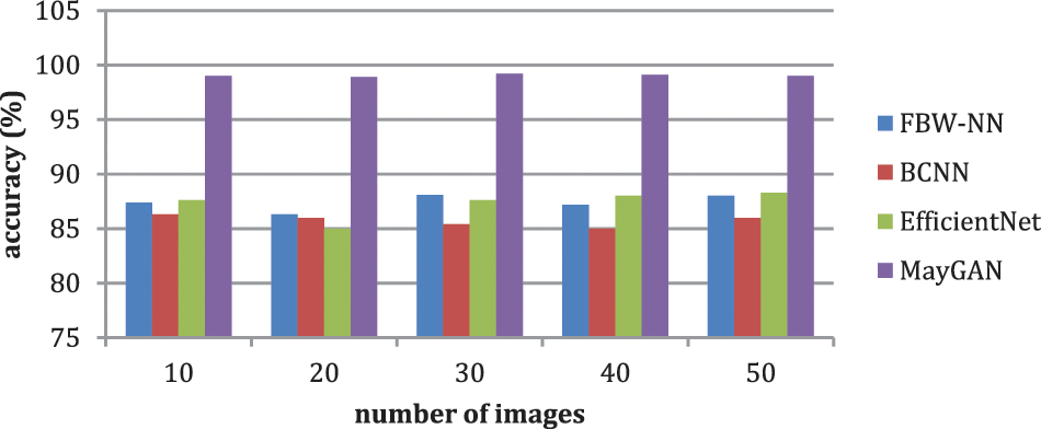
Figure 7: Analysis of accuracy

The prevailing FBW-NN, BCNN, and EfficientNet methodologies attained a recall of 91.1%, 83.2%, and 89.4%, accordingly. In correlation, the proffered MayGAN methodology attained 99.7% recall, which remains 8.6%, 16.5%, and 10.5% finer than FBW-NN, BCNN, and EfficientNet methodologies.

The prevailing FBW-NN, BCNN, and EfficientNet methodologies attained an F1-score of 93.2%, 85.6%, and 87.5%, accordingly. In correlation, the proffered MayGAN methodology attained a 97.4% F1-score that remains 4.3%, 12.2%, and 10.1% finer than FBW-NN, BCNN, and EfficientNet methodologies, accordingly. The prevailing FBW-NN, BCNN, and EfficientNet methodologies attained a DSC of 91.2%, 87.4%, and 98.6%, accordingly. In correlation, the proffered MayGAN methodology attained 98.5% DSC, remains 7.3%, 11.1%, and 0.1% finer than FBW-NN, BCNN, and EfficientNet methodologies. Table 6 shows the overall comparative analysis.

Fig. 8 indicates that the suggested MayGAN achieves 99.85% of accuracy, 98.5% of precision, 99.7% of recall, 97.4% of F1-score, and 98.5% of DSC.

Figure 8: Proposed method comparison with existing methods

5  Conclusions

Leukemia is a type of blood cancer that generally affect children and adults. The type of cancer and the extent of its dissemination throughout the body affect Leukaemia treatment. Infected patients need to receive the proper care and heal immediately, and the disease must be identified as soon as feasible. This research created an automatic diagnosis tool for four classes. Utilizing the suggested methods, the dataset was preprocessed to reduce noise and blurriness and improve image quality. This work discovered that the output photos had already been segmented during preprocessing. The strategy is valid and avoids the need for image segmentation. In order to provide help with effective feature extraction and classification, Mayfly optimization with Generative Adversarial Network (MayGAN) is introduced in this research. In addition, Generative Adversarial System is integrated with Principal Component Analysis (PCA) in the feature-extracted model to classify the type of blood cancer in the data. As a result, it is found that the proposed MayGAN achieves 99.8% of accuracy, 98.5% of precision, 99.7% of recall, 97.4% of F1-score, and 98.5% of DSC.

The suggested approach will be used in everyday life after being confirmed with significant data, assisting doctors and patients in making the earliest possible illness diagnoses. Whenever two or more stains are contacting, this suggested technique has some restrictions because these are considered one item. Therefore, future research hopes to expand our present analysis to include unstained blood smear images and enhance the sub-classification of each leukemic type based on the course of the malignancy.

Acknowledgement: The author would like to thank the Deanship of Scientific Research at Umm Al-Qura University for supporting this work by Grant Code: (22UQU4281768DSR01).

Funding Statement: This research is funded by the Deanship of Scientific Research at Umm Al-Qura University, Grant Code: 22UQU4281768DSR01.

Conflicts of Interest: The authors declare they have no conflicts of interest to report regarding the present study.

References

    1. T. TTP, G. N. Pham, J. H. Park, K. S. Moon, S. H. Lee et al., “Acute leukemia classification using convolution neural network in clinical decision support system,” in 6th Int. Conf. on Advanced Information Technologies and Applications (ICAITA 2017), Sydney, Australia, pp. 49–53, 2017. [Google Scholar]

    2. L. Perez and J. Wang, “The effectiveness of data augmentation in image classification using deep learning,” arXiv, 2017. [Google Scholar]

    3. C. N. Vasconcelos and B. N. Vasconcelos, “Convolutional neural network committees for melanoma classification with classical and expert knowledge-based image transforms data augmentation,” arXiv, 2017. [Google Scholar]

    4. S. Kansal, S. Purwar and R. K. Tripathi, “Trade-off between mean brightness and contrast in histogram equalization technique for image enhancement,” in 2017 IEEE Int. Conf. on Signal and Image Processing Applications (ICSIPA), Kuching, Malaysia, pp. 195–198, 2017. [Google Scholar]

    5. R. D. Labati, V. Piuri and F. Scotti, “All-IDB: The acute lymphoblastic leukemia image database for image processing,” in 18th IEEE Int. Conf. on Image Processing, Brussels, Belgium, pp. 2045–2048, 2011. [Google Scholar]

    6. C. Reta, L. Altamirano, J. A. Gonzalez, R. Diaz-Hernandez, H. Peregrina et al., “Segmentation and classification of bone marrow cells images using contextual information for medical diagnosis of acute leukemias,” PLOS ONE, vol. 10, no. 7, pp. 1–18, 2015. [Google Scholar]

    7. F. Kazemi, T. A. Najafabadi and B. N. Araabi, “Automatic recognition of acute myelogenous leukemia in blood microscopic images using k-means clustering and support vector machine,” Journal of Medical Signals & Sensors, vol. 6, no. 3, pp. 183–193, 2016. [Google Scholar]

    8. S. Mohapatra, D. Patra and S. Satpathi, “Image analysis of blood microscopic images for acute leukemia detection,” in Proc. of the 2010 Int. Conf. on Industrial Electronics, Control and Robotics, Rourkela, India, pp. 215–219, 2010. [Google Scholar]

    9. K. M. Garrett, F. A. Hoffer, F. G. Behm, K. W. Gow, M. M. Hudson et al., “Interventional radiology techniques for the diagnosis of lymphoma or leukemia,” Pediatric Radiol, vol. 32, no. 9, pp. 653–662, 2002. [Google Scholar]

  10. Y. Alotaibi, M. Malik, H. Khan, A. Batool, S. Islam et al., “Suggestion mining from opinionated text of big social media data,” Computers, Materials & Continua, vol. 68, no. 3, pp. 3323–3338, 2021. [Google Scholar]

  11. R. D. Labati, V. Piuri and F. Scotti, “ALL-IDB: The acute lymphoblastic leukemia image database for image processing,” in Proc. of the 2011 IEEE Int. Conf. on Image Processing (ICIP 2011), Brussels, Belgium, pp. 2045–2048, 2011. [Google Scholar]

  12. T. T. P. Thanh, V. Caleb, A. Sukhrob, L. Suk-Hwan and K. Ki-Ryong, “Leukemia blood cell image classification using convolutional neural network,” International Journal of Computer Theory and Engineering, vol. 10, no. 2, pp. 54–58, 2018. [Google Scholar]

  13. T. Karthikeyan and N. Poornima, “Microscopic image segmentation using fuzzy c means for leukemia diagnosis,” International Journal of Advanced Research in Science, Engineering and Technology, vol. 4, no. 1, pp. 3136–3142, 2017. [Google Scholar]

  14. U. R. Acharya, S. L. Oh, Y. Hagiwara, J. H. Tan and H. Adeli, “Deep convolutional neural network for the automated detection and diagnosis of seizure using eeg signals,” Computers in Biology and Medicine, vol. 100, pp. 270–278, 2018. [Google Scholar]

  15. V. J. Ramya and S. Lakshmi, “Acute myelogenous leukemia detection using optimal neural network based on fractional black-widow model,” Signal, Image and Video Processing, vol. 16, no. 1, pp. 229–238, 2022. [Google Scholar]

  16. M. E. Billah and F. Javed, “Bayesian convolutional neural network-based models for diagnosis of blood cancer,” Applied Artificial Intelligence, vol. 36, no. 1, pp. 1–22, 2022. [Google Scholar]

  17. L. F. Rodrigues, A. R. Backes, B. A. N. Travençolo and G. M. B. de Oliveira, “Optimizing a deep residual neural network with genetic algorithm for acute lymphoblastic leukemia classification,” Journal of Digital Imaging, vol. 35, no. 3, pp. 623–637, 2022. [Google Scholar]

  18. S. Chand and V. P. Vishwakarma, “A novel deep learning framework (dlf) for classification of acute lymphoblastic leukemia,” Multimedia Tools and Applications, vol. 81, no. 26, pp. 37243–37262, 2022. [Google Scholar]

  19. G. Atteia, A. A. Alhussan and N. A. Samee, “BO-ALLCNN: Bayesian-based optimized cnn for acute lymphoblastic leukemia detection in microscopic blood smear images,” Sensors, vol. 22, no. 15, pp. 5520, 2022. [Google Scholar]

  20. D. Baby, S. Juliet and M. M. Anishin Raj, “An efficient lymphocytic leukemia detection based on efficientnets and ensemble voting classifier,” International Journal of Imaging Systems and Technology, pp. 1–8, 2022. [Google Scholar]

  21. C. Mondal, M. Hasan, M. Jawad, A. Dutta, M. Islam et al., “Acute lymphoblastic leukemia detection from microscopic images using weighted ensemble of convolutional neural networks,” arXiv preprint arXiv: 2105.03995, 2021. [Google Scholar]

  22. F. S. K. Sakthiraj, “Autonomous leukemia detection scheme based on hybrid convolutional neural network model using learning algorithm,” Wireless Personal Communications, vol. 126, no. 2, pp. 2191–2206, 2022. [Google Scholar]

  23. M. Z. Ullah, Y. Zheng, J. Song, S. Aslam, C. Xu et al., “An attention-based convolutional neural network for acute lymphoblastic leukemia classification,” Applied Sciences, vol. 11, no. 22, pp. 10662, 2021. [Google Scholar]

  24. Z. Jiang, Z. Dong, L. Wang and W. Jiang, “Method for diagnosis of acute lymphoblastic leukemia based on vit-cnn ensemble model,” Computational Intelligence and Neuroscience, vol. 2021, no. 9, pp. 1–12, 2021. [Google Scholar]

  25. M. Ghaderzadeh, F. Asadi, A. Hosseini, D. Bashash, H. Abolghasemi et al., “Machine learning in detection and classification of leukemia using smear blood images: A systematic review,” Scientific Programming, vol. 2021, no. 5, pp. 1–14, 2021. [Google Scholar]

  26. Y. Alotaibi and A. F. Subahi, “New goal-oriented requirements extraction framework for e-health services: A case study of diagnostic testing during the COVID-19 outbreak,” Business Process Management Journal, vol. 28, no. 1, pp. 273–292, 2022. [Google Scholar]

  27. J. Jayapradha, M. Prakash, Y. Alotaibi, O. I. Khalaf and S. A. Alghamdi, “Heap bucketization anonymity—An efficient privacy-preserving data publishing model for multiple sensitive attributes,” IEEE Access, vol. 10, pp. 28773–28791, 2022. [Google Scholar]

  28. Y. Alotaibi, “A new meta-heuristics data clustering algorithm based on tabu search and adaptive search memory,” Symmetry, vol. 14, no. 3, pp. 623, 2022. [Google Scholar]

  29. K. Lakshmanna, N. Subramani, Y. Alotaibi, S. Alghamdi, O. I. Khalaf et al., “Improved metaheuristic-driven energy-aware cluster-based routing scheme for IoT-assisted wireless sensor networks,” Sustainability, vol. 14, no. 13, pp. 7712, 2022. [Google Scholar]

  30. S. S. Rawat, S. Alghamdi, G. Kumar, Y. Alotaibi, O. I. Khalaf et al., “Infrared small target detection based on partial sum minimization and total variation,” Mathematics, vol. 10, no. 4, pp. 671, 2022. [Google Scholar]

  31. M. Abdel-Fattah, O. Al-marhbi, M. Almatrafi, M. Babaseel, M. Alasmari et al., “Sero-prevalence of hepatitis B virus infections among blood banking donors in Makkah city, Saudi Arabia: An institutional-based cross-sectional study,” Journal of Umm Al-Qura University for Medical Sciences, vol. 6, no. 2, pp. 4–7, 2020. [Google Scholar]

  32. A. A. Malibari, M. Obayya, M. K. Nour, A. S. Mehanna, M. Ahmed Hamza et al., “Gaussian optimized deep learning-based belief classification model for breast cancer detection,” Computers, Materials & Continua, vol. 73, no. 2, pp. 4123–4138, 2022. [Google Scholar]

  33. N. Dilshad, A. Ullah, J. Kim and J. Seo, “LocateUAV: Unmanned aerial vehicle location estimation via contextual analysis in an IoT environment,” IEEE Internet of Things Journal, vol. 99, pp. 1, 2022. [Google Scholar]

  34. M. Usman, T. Saeed, F. Akram, H. Malaikah and A. Akbar, “Unmanned aerial vehicle for laser based biomedical sensor development and examination of device trajectory,” Sensors, vol. 22, no. 9, pp. 3413, 2022. [Google Scholar]

  35. U. Masud, F. Jeribi, M. Alhameed, F. Akram, A. Tahir et al., “Two-mode biomedical sensor build-up: Characterization of optical amplifier,” Computers, Materials & Continua, vol. 70, no. 3, pp. 5487–5489, 2022. [Google Scholar]

  36. U. Masud, F. Jeribi, M. Alhameed, A. Tahir, Q. Javaid et al., “Traffic congestion avoidance system using foreground estimation and cascade classifier,” IEEE Access, vol. 8, pp. 178859–178869, 2020. [Google Scholar]