Statistical Time Series Forecasting Models for Pandemic Prediction

1  Introduction

Infectious diseases are the leading cause of human mortality around the world. The occurrences of infectious diseases can be traced back to the Middle Ages. COVID-19, an unusual coronavirus, was discovered in Wuhan, China, in December 2019. The newly identified virus has been linked to 470 million confirmed infections [1]. Vaccinations for SARS-CoV-2 and antiviral measures such as wearing masks and avoiding large crowds are critical in preventing viral spread. Many vaccines have shown the efficacy of more than 95% in preventing SARS-CoV-2 symptoms. Approximately 80 M COVID-19 infections and 1 M coronavirus-related fatalities have been reported in the USA alone [1]. Diverse mathematical epidemic surveillance models [2–4] have been given in the literature [2]. Biological and disease mechanisms that use epidemiological methodologies are important in most modeling approaches to predict the progression of outbreaks and pandemics.

An effective method of accomplishing this is accurately predicting the number of active cases at any time. Time-series data include confirmed daily COVID-19 cases, recoveries, and deaths, to name a few instances. Time-series data are a series of numeric values measured at intervals equal in length (e.g., per minute, hour, or day) [3]. To anticipate the future dynamics of influenza, malaria tuberculosis, and other infectious diseases [4,5], different time series models were utilized to forecast COVID-19 in the United States, Italy, India, and other countries [6].

Despite this, no general concept for selecting models for projecting the spread of COVID-19 has been established. It is also recommended that multiple models can be used to forecast the spread of the epidemic in different states and under different conditions of the pandemic propagation. Deep learning models, for example, were demonstrated in [7] to have the lowest rates of forecast errors while tracking the dynamics of infection cases in the four nations under consideration [7,8]. The following are the main significant advantages of ARIMA:

(1)   Dealing with tiny data.

(2)   Being simple to implement with no parameter adjusting.

(3)   Being easier to handle multivariate data.

(4)   Being quick to run.

In addition, the following are some of the characteristics of deep learning models:

(1)   There are no pre-requisites (stationarity, no level shifts).

(2)   Neural networks can model nonlinear functions.

(3)   Requires a large amount of data (Big Data).

(4)   Time-series models are considered more appropriate for dealing with COVID-19 data because they can deal with small amounts of data.

In this paper, the proposed methodology uses various data published across the globe for the active cases of patients identified with coronavirus infection (in this example), the total number of deaths recorded due to the virus impact, and the total number of cases that have been recovered. To ensure the precision of the Artificial Intelligence (AI) models, epidemiological time series are employed to monitor and manage the spread of infection and its containment. In addition, this work intends to investigate various ways to forecast an outbreak and identify abnormalities in historical data. This may be used without compromising the data accuracy, or periodicity, assisting management of the regions to combat the spread of infection.

As a result, data analytics and ML techniques may be used to develop a more comprehensive understanding of viruses. A comparative review of COVID-19 forecasting models, including ML techniques, is presented in this paper, along with examining the distribution and transmission of COVID-19 in various nations. Thus, this research has examined the empirical performance of several classical univariate time series models, as well as ML-based regression algorithms such as Logistic Regression, Lasso, Ridge, ElasticNet, Huber Regressor, Lasso Lars, K-Neighbors Regressor, Passive Aggressive Regressor, Random Forest Regressor, Extra Trees Regressor, SVR, AdaBoost Regressor, Bagging Regressor, Decision Tree Regressor, Gradient Boost, Croston, and NaiveBayes.

The following sections are organized as follows. First, a literature survey for some of the recently published related studies is introduced. The next section includes data description materials and methods. Subsequently, the discussion of modeling and forecasting outcomes are presented. The final section provides the recommendations, conclusions, and future works.

2  Related Work

The purpose of time series forecasting as an asset is to ease the forecasting process and to create a convenient and easy-to-use application/tool for any kind of situation dealing with the need to have a futuristic visualization of the trend of the data involved in the planning of any domain.

COVID-19 scatter forecasting, or simply future impact projection, provides essential inputs for government, public health agencies, corporations, and citizens to schedule, organize, and manage an outbreak. As a result, most outbreak models used in the tracking and forecasting of COVID-19 are based on epidemiological patterns, such as susceptible, infected, and eliminated individuals [8]. The Susceptible-Exposed-Infected-Removed (SEIR), Susceptible-Exposed–Infected–Recovered–Dead (SEIRD), and extended Susceptible–Infected–Removed (SIR) [9] models incorporate variable-time quarantine procedures such as macro-isolation rules at the federal level and standard isolation policies. To forecast infection, several AI-based models have been published in the literature. These models include an interior searching algorithm and a multi-layer Artificial Neural Network (ANN) feedforward. Several trends in this field include the following models [10]: (1) modified stacks for transmission dynamics, (2) nonlinear hybrids for predicting affected, (3) recovered and lethal molecules, (4) agent-based AI simulation platform (EnerPol) for predicting growth and containment strategy, (5) multi-input deep convolutional neural network (CNN) for predicting the cumulative number of confirmed cases, (6) topological autoencoder for generating a similarity map of transmission dynamics, and (7) SEIR.

The work in [11] explores the contemporary pattern or trend of COVID-19 transmission in any highly impacted country like India and the regression analysis of other data (like different information for Indian data). In their work, five models were used in this study: Linear Regression (LR), Exponential Smoothing (ES), K-Nearest Neighbors (KNN), Random Forest (RF), and Support Vector Machines (SVM). Each model contains two types of predictions: (1) a newly positive number of eases verified and (2) several people killed.

In research conducted by author in [12], the authors have developed a new nonlinear deterministic model based on ordinary differential equations with six compartments, quarantine, and isolation. The model has a positive invariant area, while the balance points are investigated concerning the simple reproductive number in terms of its local stability. Furthermore, a new mathematical model for predicting the spreading of epidemics in Egypt has been suggested in [13]. In the proposed model, the number of cases was raised significantly after two months, concluded from exploring the data. Consequently, a series of proliferation prevention initiatives had to be adopted, such as implementing systematic prohibition, isolation, and social divergence policies over a specific timeframe.

Many researchers have attempted to forecast the outbreak of COVID-19 by using diverse mathematics methods like the classic SIR model and its derivatives [14–20]. This analysis simulated the outbreak from February 14 to April 11 in Isfahan Province of Iran and predicted the remaining direction with three different socially distinguishing scenarios. To anticipate the pandemic, further advanced models and a detailed understanding of the epidemic biomedical and epidemiological dimensions were needed [14].

In summary, the pandemic characteristics of COVID-19 are inconsistent with the SIR modeling system. For most of which quantitative evidence is not yet available, the mechanisms of this epidemic were subject to different parameters. The new approach suggested produced improved outcomes and showed the value of social distance [15]. Their research proposed ML and deep learning (DL) algorithms such as Long Short-Term Memory (LSTM), eXtreme Gradient Boost, and polynomial regression in forecasting to estimate COVID-19 count in advance and enhance precision [16].

To find out the forecast for the upcoming months, the whole data should be used to check for the pattern and stationarity of the data. The outliers can be treated using either Mean-Standard Deviation (MSD) or Median Absolute Deviation (MAD) [17]. According to [18], not much research was done on this particular application (to have thorough research on all the time series, ML, and deep learning models for the forecasting problem) using the different ML techniques. Once implemented, this algorithm could be used in any domain such as heart rate measurement, climate changes, forecasting of foods, sales of retail industries, etc. [19]. The researchers presented some of the well-known models used widely for forecasting demand, and an extensive comparison of their performances is made, and inferences are drawn [20–25]. Many different models are available in the research fields that vary from the statistical time series algorithms and regression-based ML algorithms rather than deep learning-based algorithms like the LSTM [21].

The methods used to determine and compare the results of Canadian Foundries’ orders are NN, RNN, and SVM [22]. In [23], many statistical approaches like the ARIMA are used along with the Artificial Neural Networks (ANNs) to use the linearity of the ARIMA and nonlinearity of the ANNs to make a hybrid model. The same was also proven in [24], so the linear and the nonlinearity of the data can be captured. The hybrid model or the ensemble of several models is standard for better accuracy since the well-known M-competition [24].

Various studies have been done to understand combining the models to give a better forecast. In an analysis of the time-series data, which has a powerful trend and seasonality, a comparative study is done with the ANN and other traditional methods, including the Winters Exponential Smoothing, Box-Jenkins ARIMA model, and multivariate regression [25]. In [26], the authors focused on the extensive work on analyzing the time series, ML-based regression models, and deep learning to combine in ensemble methods. A lot of algorithms such as Auto-Regressive time series models, also known as AR models, Simple Moving Average (SMA), Simple Exponential Smoothing (SES), Weighted Moving Average (WMA), and Holts-Winter Exponential Smoothing (HWES) models [27] are used. Some naïve forecasting techniques also impact forecast generation through the time series models. The ML models can be classified into linear and nonlinear models. Some of the algorithms that are used in the linear ML regression models are Linear (LR), Lasso, Ridge, Elastic Net (EN), Huber, Lasso Lars (LLARS), Passive-Aggressive (PA), and regression models. Also, in the case of the nonlinear ML regression models, K-Neighbors, Decision Tree, Extra Tree, SVR, AdaBoost, Bagging, Random Forest, Extra Trees, and Gradient Boosting regressor models are used. In addition, deep learning models such as LSTMs and Multilayer Perceptron (MLP) [28,29] are used.

3  Methodology

The goal of implementing the time series forecasting algorithm is to create genericity of the modeling, which gives better accuracy and presents a highly stable prediction model that generates reliable forecasts for any relevant data type. In this work, we concentrate on assembling with a weighted average as the second level learner.

3.1 Basic Steps of Time Series Forecasting

3.1.1 Data Input

The model will automatically grasp weekly, monthly, quarterly, and annual data based on the type of input data with information in the time domain. As a result, the model will produce the output. The outcome might be made based on the requirements of the research fields. During the input data procedure, the data, which is time-constrained country-wise monthly data, is used to evaluate the model performance. The features or current information in the coronavirus-based country-wise monthly dataset are the various routes via which the virus impact is to be studied and traced. Additional information that can be used to report the overall virus impact includes the Region, City, State, Country, and the general Continent and Global Level. Various steps are taken to put the data in the appropriate shape to carry out the forecasting task. According to the Data Sharing Agreement (DSA) [21], the data should be profiled to cluster out the original dataset to the specific cluster in which a better algorithm can make the forecast.

3.1.2 Data Pre-Processing

•   Imputation of Null values: This will be done through nearest points imputation. In contrast to traditional imputation techniques that take into account imputing with the mean, maximum, median, and so on, a different approach is used here.

•   Removal of Outliers: The global impacted data is very susceptible to outliers because of the introduction of many government measures that affect the real amount. As a result, these values must be processed before being entered into the model. Some of the strategies include determining the seasonality pattern or employing basic mean-standard deviation or median absolute deviation deductions [30].

•   Formulation of Datasets: Because the data consists of single column values, it must be transformed into a dataset before being fed into ML regression-based models. A tree-based approach considers delays. The p-value is used as an input for the lags generation in the ARIMA model, which has different hyper-parameters. Finally, the supervised learning dataset is created for the ML regression models.

•   Check for Stationarity: The dataset can be made stationary using the dickey-fullers test [28].

•   Data Scaling: The process of causing a dataset to fall into a specific interval for ML models to perform properly.

3.1.3 Forecast Generation

The processed dataset is fed into time series, ML, and deep learning forecasting algorithms to generate trained models that understand the fluctuation in the training dataset history sample set.

Sub-Step 1: Creating Validation Samples: Training and testing sets are constructed to evaluate the model performance. The Hold-Out strategies of 60%–40%, 70%–30%, or 80%–20% of the total dataset are employed for the sample sets. Root Mean Squared Error (RMSE) is used for tuning and error minimization. The error is then checked in the validation or testing sets to ensure that the model behavior and stability are correct.

Many statistical and ML-based time series forecasting models are considered in our proposed methodology, such as ARIMA, ARMA, moving average (MA), Weighted Moving Average (WMA), Holts-Winters, Croston, Linear Trend, Naive Forecast, as statistical time series algorithms and Linear Regression, Decision Tree Regression, SVR, Passive Regression as ML-based algorithms amongst many others. The best model produces the least amount of error when verifying the sample set generated above.

Sub-Step 2: Collection of the above algorithms: The errors produced from the statistical time series and ML-based regression models, developed in the previous steps, create the respective weights for the separate algorithms.

3.1.4 Ensemble Weights Assignments

The best of each of the models is then input into the ensemble model to find the best results. The weights that are assigned to each of the models (wts, wml, wdl) are calculated as follows [31].

wts=1errorts/(1errorts+1errorml+1errordl)(1)

wml=1errorml/(1errorts+1errorml+1errordl)(2)

wdl=1errordl/(1errorts+1errorml+1errordl)(3)

3.1.5 Final Forecast Generation

The next step is to consider the forecast generation for future periods. Throughout this methodology, we will consider the following factors: improve forecasting or forecast accuracy, detect future patterns, and forecast models’ forecast stability. The model stability means that “if Model 1 is selected,” the same model should continually perform well without fluctuating accuracy. This scenario will consider three historical data points for a five-month rolling projection.

3.2 Statistical and AI-Based Forecasting Models

3.2.1 Logistic Regression Algorithm

Logistic regression is a linear model (which seeks to linearly fit the hyperplane) that attempts to predict the likelihood of an event occurring. A binary dependent variable is modeled using a sigmoid or logit function. In this situation, it optimizes the cost function (error curve in the bowl-shaped plane), which is the Mean Squared Error (MSE) or the model accuracy of the predictions, to minimize error and achieve optimal weights [25].

3.2.2 Random Forest Classifier

It is a classification algorithm made up of numerous decision trees. Building each individual tree employs bagging and feature randomness to produce an uncorrelated forest of trees [14].

3.2.3 AdaBoost Classifier

It utilizes an iterative approach to learn from the errors of weak classifiers and transform them into strong ones [32].

3.2.4 Naïve Bayes Classifier

It is a probabilistic classifier that depends on the Bayes theorem. The theorem states the likelihood of an occurrence is based on the previous or future information taken into account to characterize the event.

3.2.5 KNN Classifier

The KNN algorithm is a data categorization approach that estimates the likelihood that a data point will belong to one of two groups based on which data points are closest [23].

3.2.6 Decision Tree Classifier

Decision trees employ various techniques to determine whether to split a node into two or more sub-nodes [19].

3.3 Time Series Algorithms

3.3.1 Autoregressive Integrated Moving Average (ARIMA) Model

The following is a breakdown of the various parts of an ARIMA model:

•   It is an autoregressive (AR) model in which a variable lag or regresses prior values.

•   When the raw observations are differentiated, this is what is meant by “integrated” (I).

•   In ARIMA, each element serves as a parameter denoted by a common notation. For ARIMA models, the usual notation would be ARIMA with the parameters replaced by integer values (p, d, and q). The following are the parameters: (p) Lag order, (d) Degree of difference, and (q) Moving average window size.

•   These parameters can be determined by:

•   Autocorrelation Function (ACF) [31]: A correlation measurement between the time series and lagged time series version. The optimum amount of q words can be determined by using the ACF.

•   Partial Autocorrelation Function (PACF) [27]: After excluding the differences which are already clarified by the intermediate contrast. This tests the similarity between the time series and a lagged time series version.

3.3.2 Exponential Smoothing

A time series forecasting method for univariate data that does not have a trend or seasonality is known as Single Exponential Smoothing (SES) [31]. This method depends on a single parameter, α, which is sometimes referred to as the smoothing factor or coefficient [31].

3.4 Analysis and Evaluation Criteria

Since many regression-based algorithms are employed, some evaluation metrics are selected to measure their performance. The metrics are Mean Absolute Percentage Error (MAPE), Mean Squared Error (MSE), and Forecast Accuracy and Confidence in Forecasting (FACC) [26].

3.5 Proposed Framework Design

The proposed methodology for time series forecasting includes a comparison of statistical vs. ML-based prediction algorithms, as shown in Fig. 1.

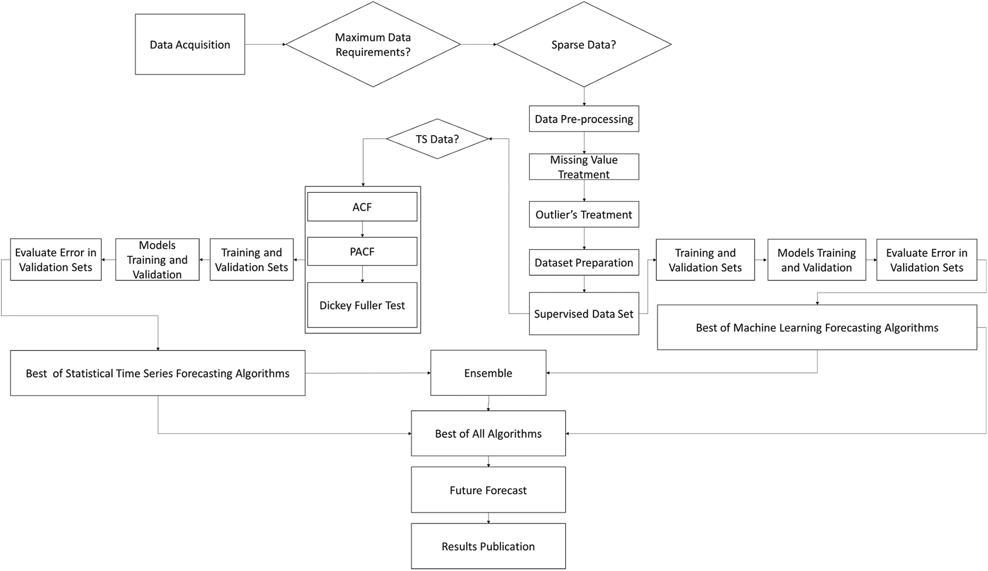
Figure 1: Proposed framework

In this regard, we have simulated, adjusted, and fitted several statistical time series forecasting models, linear ML models, and nonlinear ML models such as Logistic Regression, Lasso, Ridge, ElasticNet, Huber Regressor, Lasso Lars, Passive Aggressive Regressor, KNeighbors Regressor, Decision Tree Regressor, Extra Trees Regressor, SVR, AdaBoost Regressor, Random Forest Regressor, Bagging Regressor , AR, Gradient Boosting Regressor, ARMA, ARIMA, SES, Exponential Smoothing, Holt-Winters, Simple Moving Average, Weighted Moving Average, Croston, NaïveBayes. Furthermore, our proposed methodology includes implementing and evaluating ensemble models built on top of the best-performing statistical and ML-based prediction algorithms. A final step is added to the framework that evaluates all three implementations to determine which one provides the best performance to use the best algorithm for future forecasts. This is done to ensure that we can obtain the most accurate and reliable predictions, which could then be published on the research portal for everyone benefit.

3.6 Dataset

Our experiments focused on different COVID-19 cases which are recovered and deaths cases in five different countries of various geographical areas (United States of America, Canada, India, Australia, and United Kingdom. Each time series is divided into validation group (20%), training group (70%), and testing group (10%) [19].

4  Results and Discussion

Numerical experiments on numerous datasets from various nations have been conducted to evaluate the suggested method and demonstrate the generalizability of the designed scheme. As clarified in Fig. 2, the confirmed dataset of the monthly mean resample is depicted in green, and the original data is displayed in blue. As a result, we need to determine whether or not the dataset is stationary at this point, as clarified in Fig. 3.

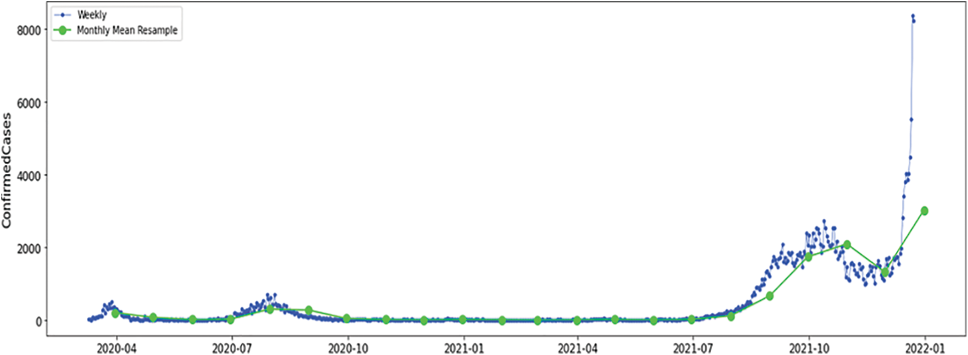
Figure 2: Confirmed cases (weekly and monthly average), Australia

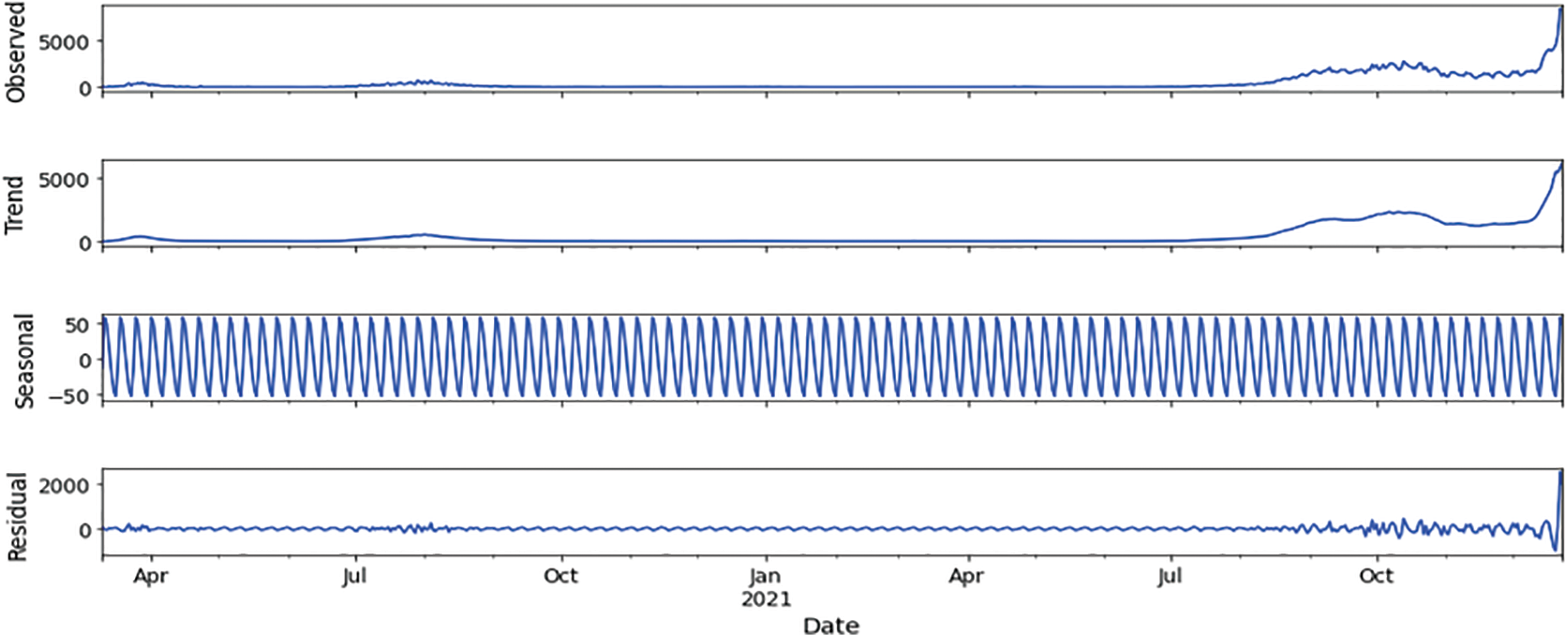
Figure 3: Decomposition of confirmed cases, Australia

When the statistical characteristics of a dataset, such as the mean, variance, and autocorrelation, remain constant across time, the dataset is said to be stable. According to Fig. 4, the augmented Dickey-Fuller test is applied to verify whether the dataset is stationary or not. Detrending, differencing, or a combination of the two is used to complete the rationalization of our dataset, as indicated in the accompanying Figs. 5–7.

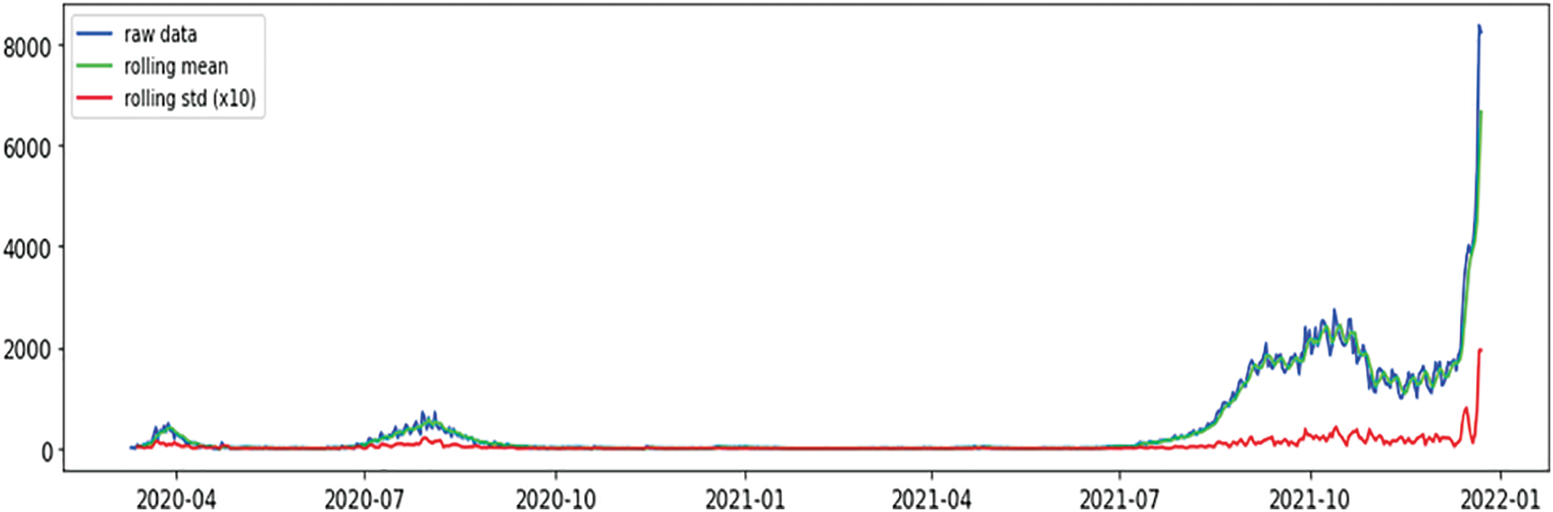
Figure 4: Mean & variance of confirmed instances

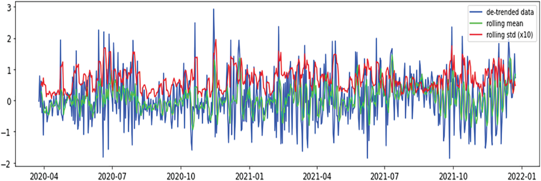
Figure 5: Mean & variance of detrended instances

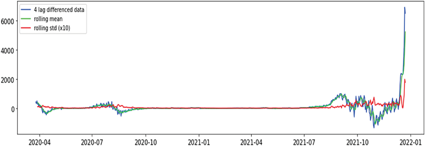
Figure 6: Mean & variance of differenced instances

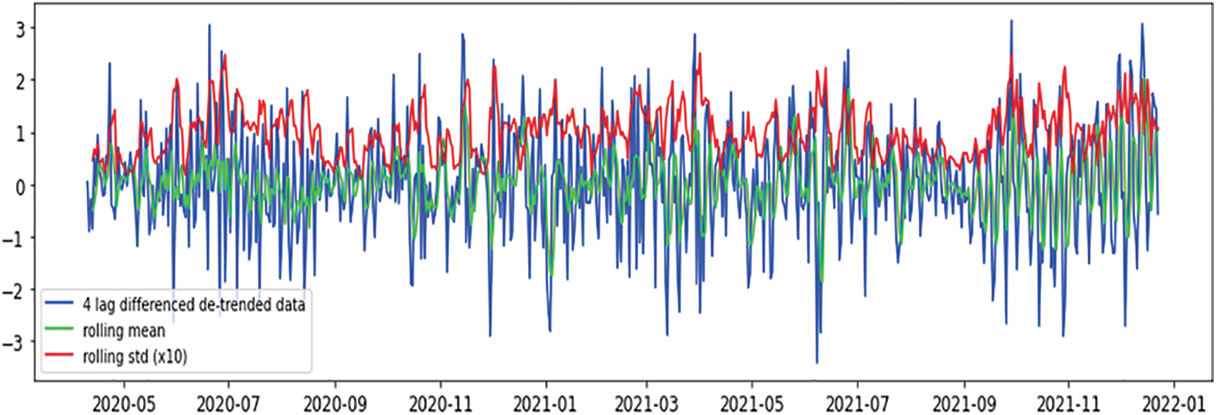
Figure 7: Mean & variance of detrended and differenced instances

The same analysis is performed for all of the five countries under examination to get the best stationary data inputs that will help increase the accuracy of the predictions, as shown in Figs. 8 and 9. We only choose to present confirmed case modeling and forecasting results to keep our research as abbreviated as possible. We found that SES, Holt, Holt-Winters, and ARIMA perform best. Amongst many ML-based forecasting models, we found that RegressionTrees, ExtraTrees, and K-Nearest Neighbor give the best forecasts.

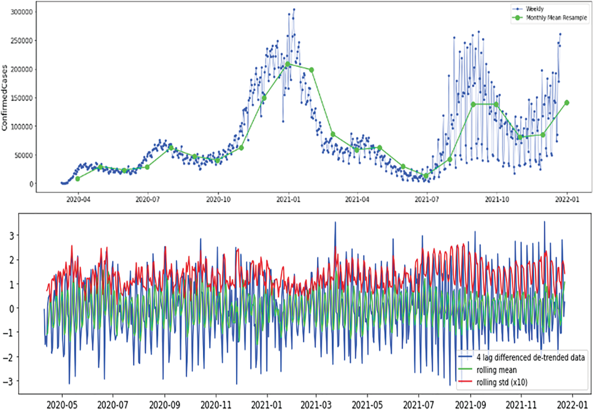
Figure 8: USA (original vs. stationary time series), mean & variance of detrended and differenced instances

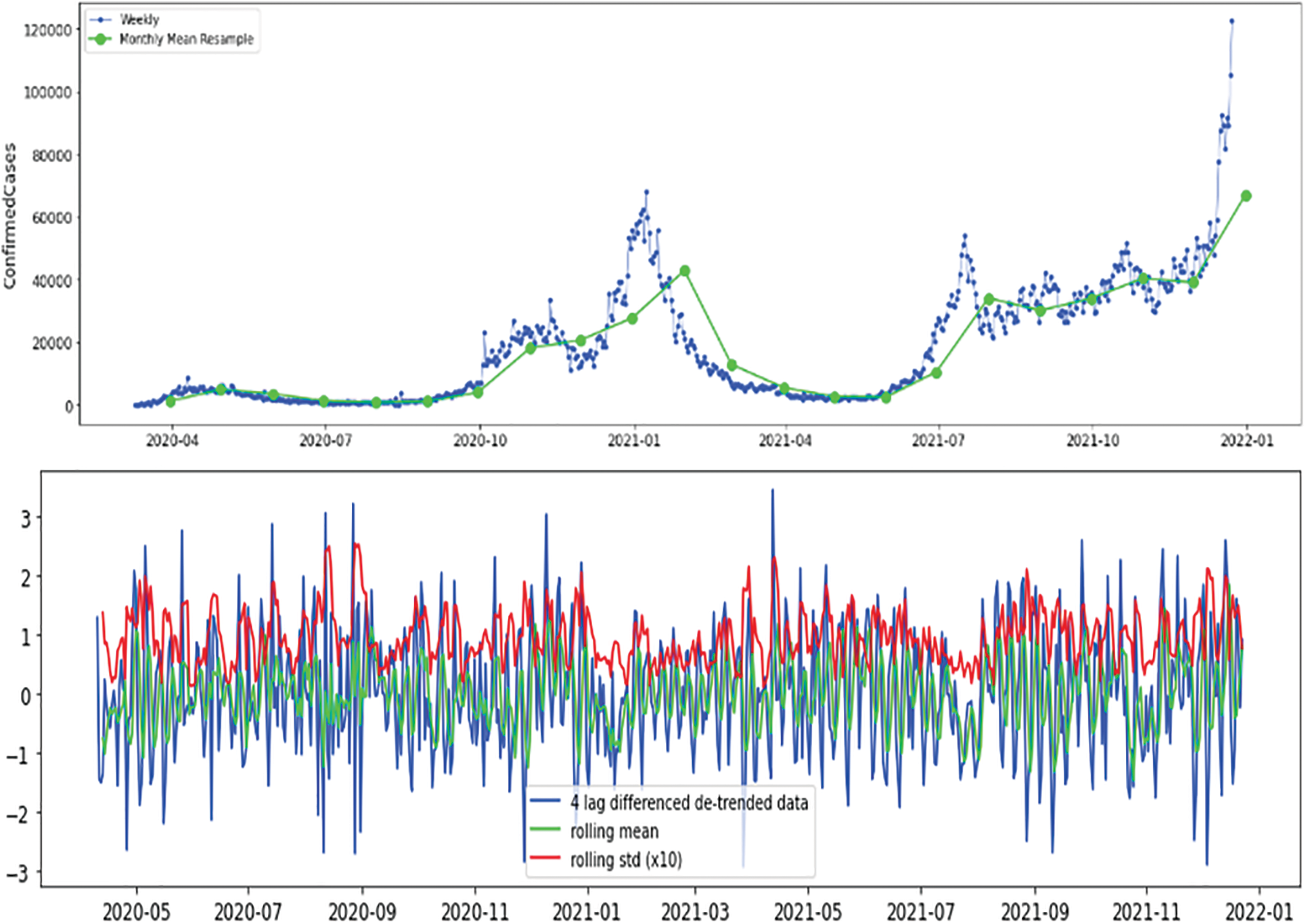
Figure 9: UK (original vs. stationary time series), mean & variance of detrended and differenced instances

Below is a graphical representation of the best-fitted model for each country. Training and validation datasets observed actuals against forecasted are visualized in Figs. 10, 14, 18, 22, 26 for Australia, Canada, India, UK, and US, respectively. From these figures, it is obvious that the COVID-19 epidemic has propagated differently for each geolocation. This could be a result of differentiated weather and population demographics.

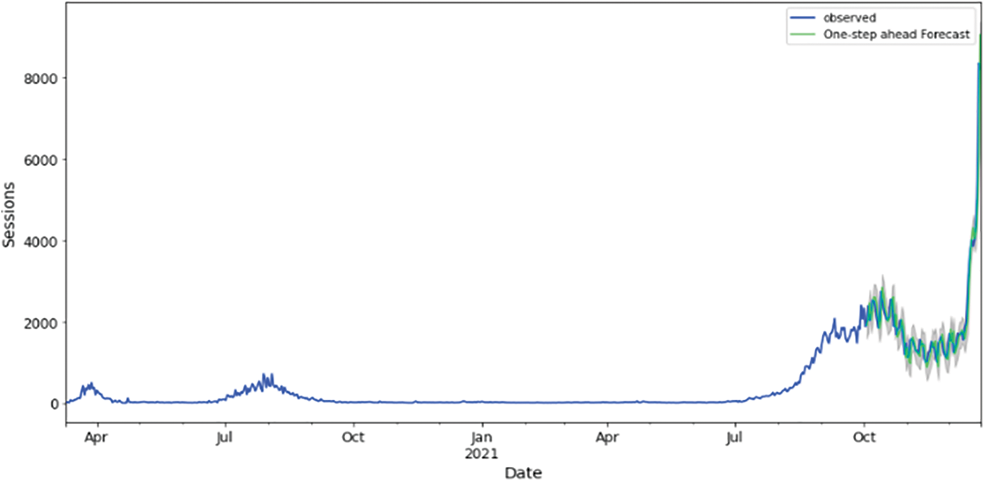
Figure 10: Training and validation datasets best fitting (best performing algorithm for Australia), HUBER ML algorithm

Figs. 11, 15, 19, 23, and 27 depict the five days forecasts for confirmed cases using the best performing ML/TS algorithms mentioned above for Australia, Canada, India, UK, and US, respectively. The graphs show a comparison between the actual observations of the confirmed case count in the period from 18th December to 23rd December and the different forecasts resulting from the best performing ML and statistical time series models, along with the forecasts obtained upon the implementation of ensemble and the weighted ensemble of these outperforming models. The corresponding RMSE for the best-performing forecasting models mentioned above is depicted in Figs. 12, 16, 20, 24, and 28 for Australia, Canada, India, UK, and US, respectively. In addition to the RMSE measure, the results from diagnostics utilizing the plot diagnostics technique are utilized to guarantee that none of the model assumptions are broken and that no out-of-the-ordinary behavior occurs.

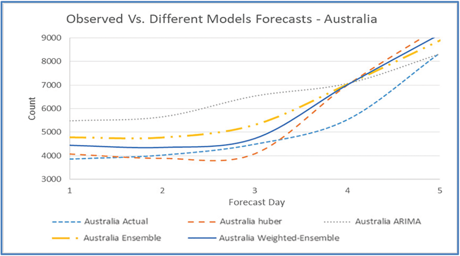
Figure 11: Five days forecast for Australia’s confirmed cases using the best performing ML/TS algorithms

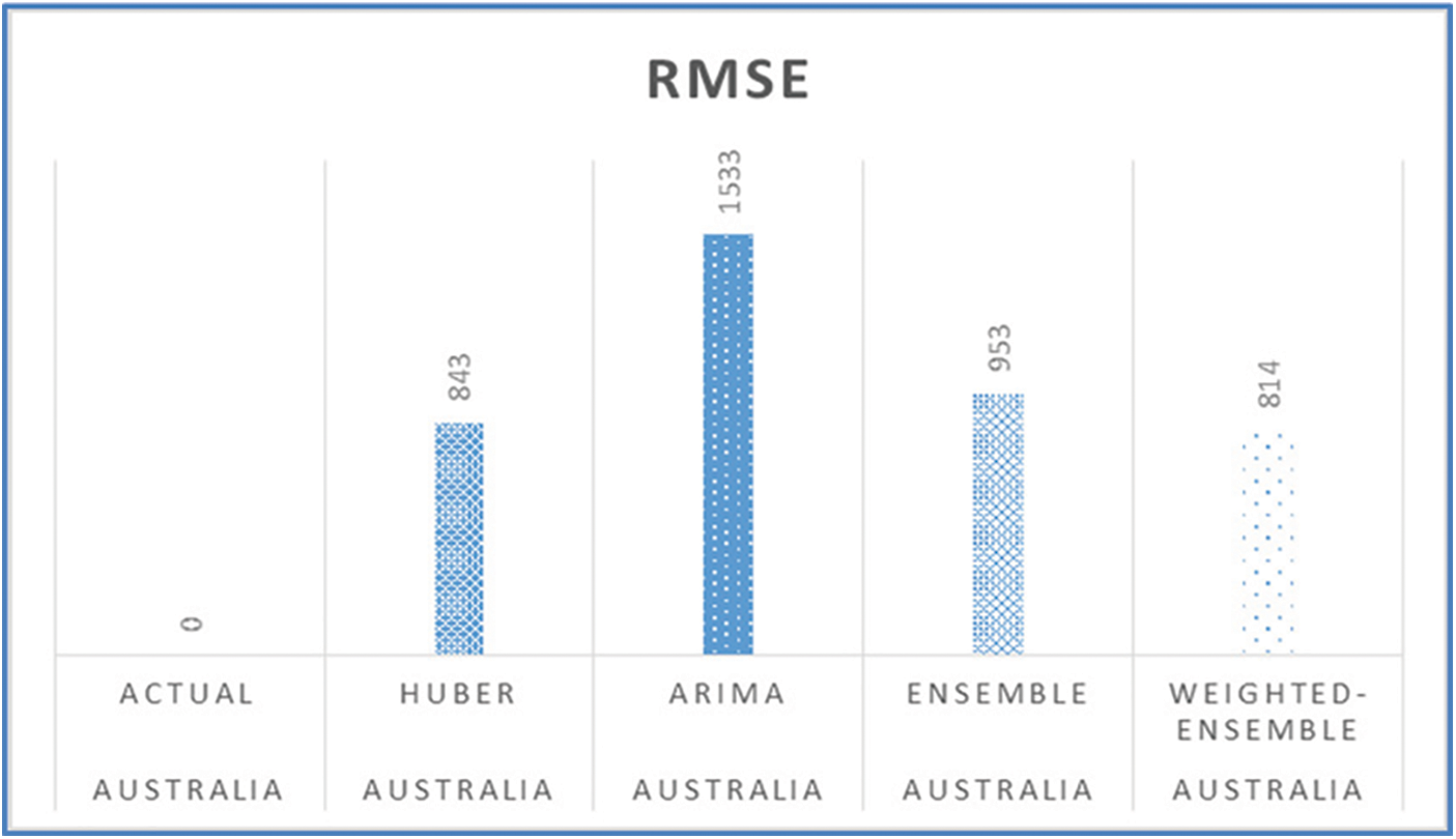
Figure 12: RMSE of the five-days forecast for Australia’s confirmed cases using best-performing models

This technique results in the four visual outputs depicted in Figs. 13, 17, 21, 25, 27, and 29 for Australia, Canada, India, UK, and US, respectively. The autocorrelation graph on the bottom right shows that the time series residuals are weakly correlated with their lag-adjusted counterparts. However, by proving all four of the arguments stated above, one can conclude that the residuals of this model are almost normally distributed. This signifies that we have found a well-suited model for our dataset.

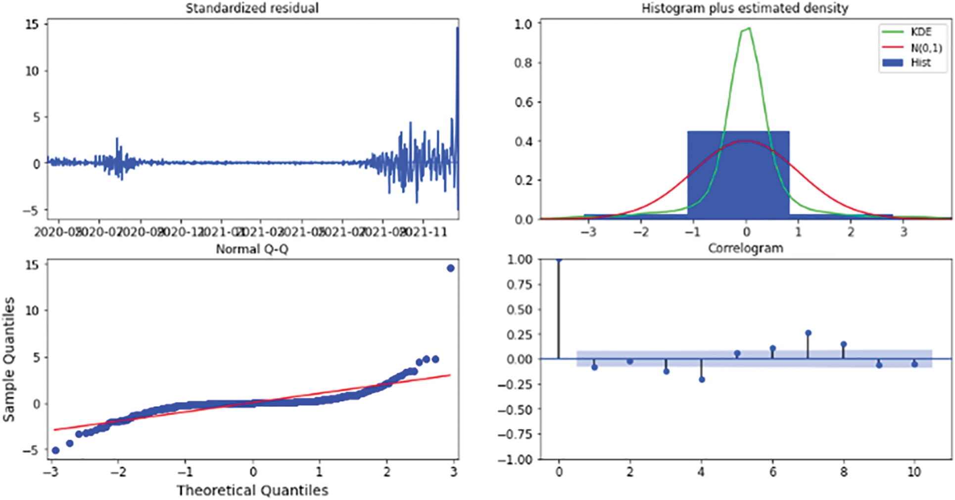
Figure 13: Results diagnostics for the five-days forecast for Australia’s confirmed cases using the weighted ensemble algorithm

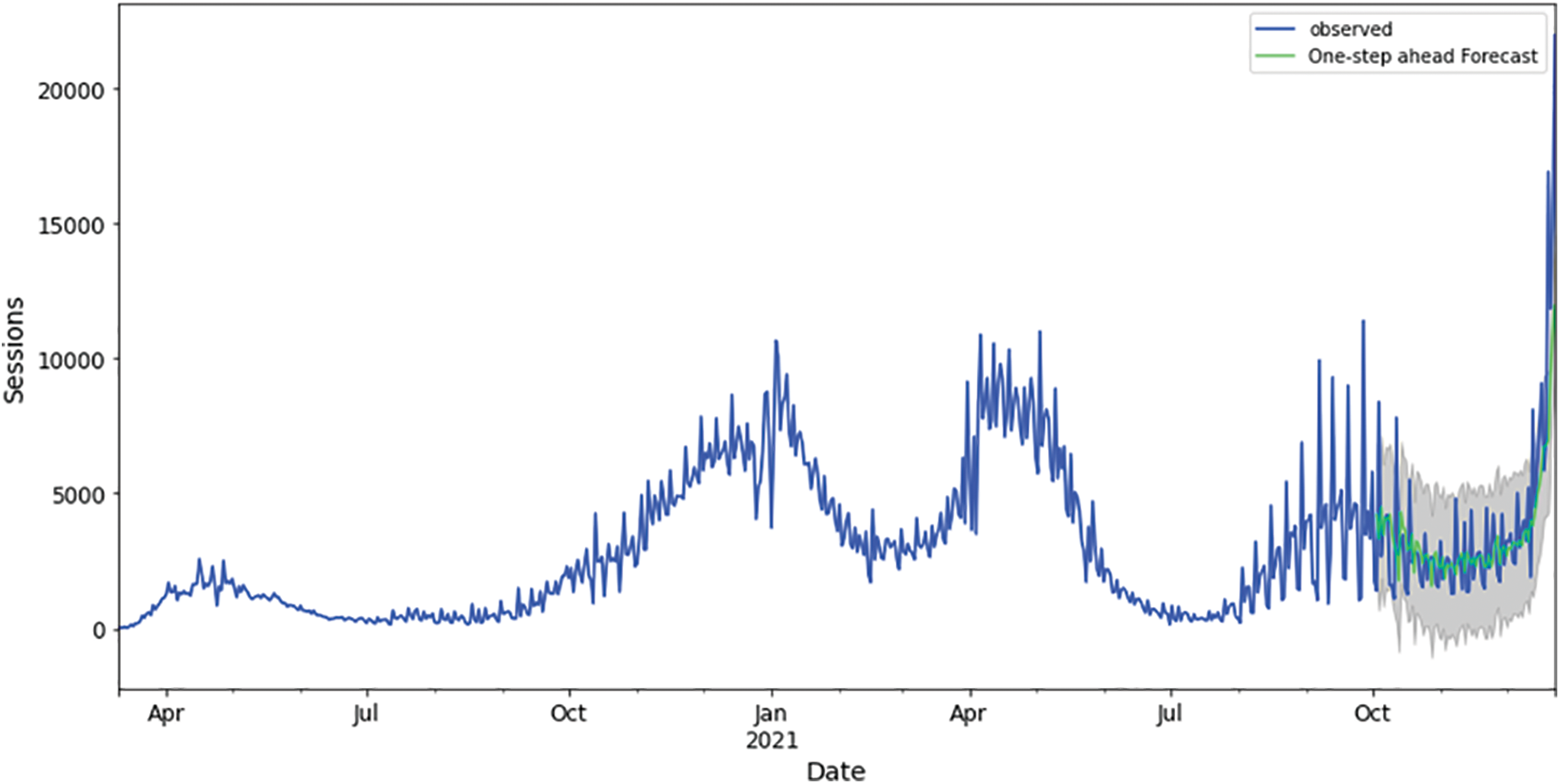
Figure 14: Training and validation datasets best fitting (best performing algorithm for Canada), KNN ML algorithm

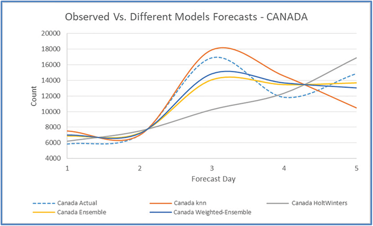
Figure 15: Five days forecast for Canada’s confirmed cases using the best performing ML/TS algorithms

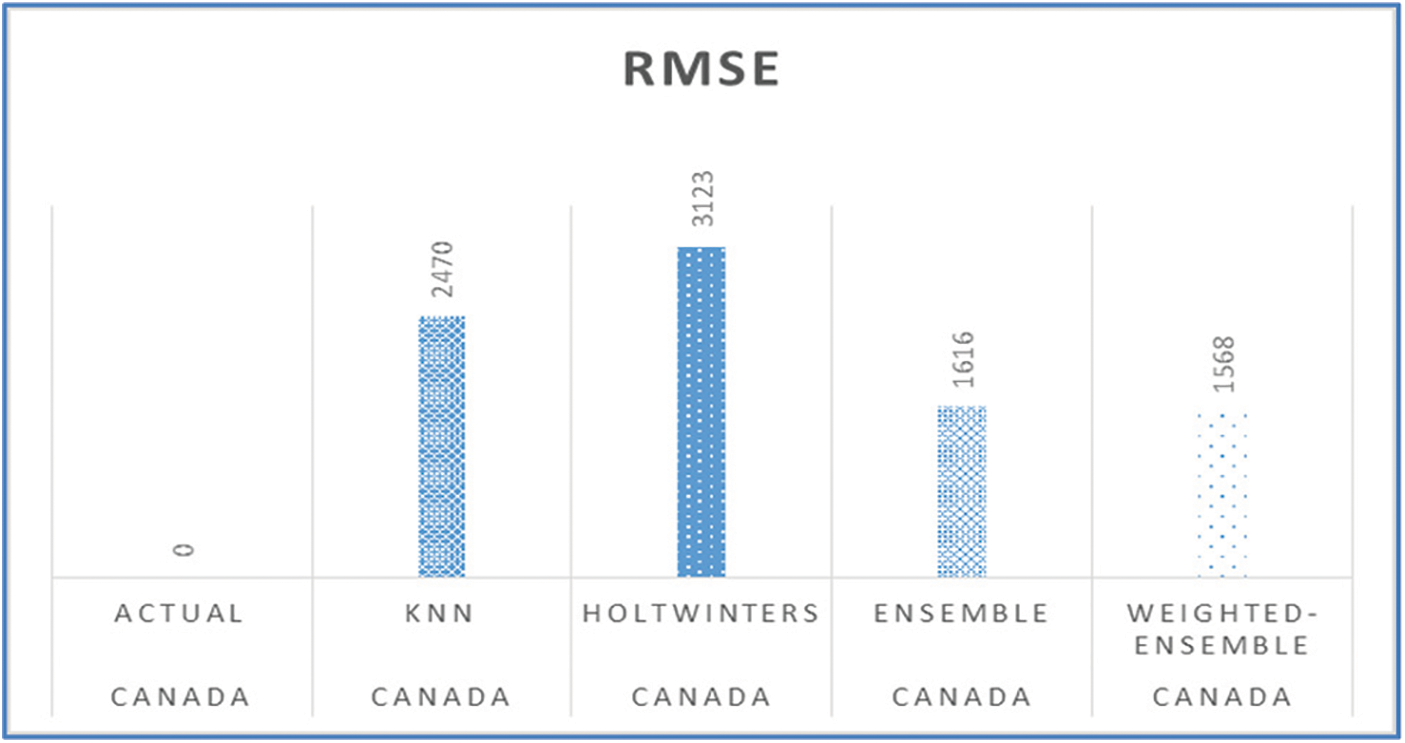
Figure 16: RMSE of the five-days forecast for Canada’s confirmed cases using best-performing models

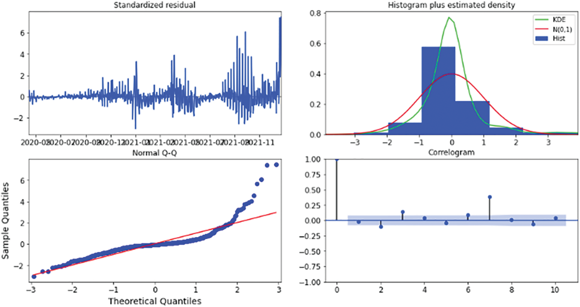
Figure 17: Results diagnostics for the five-days forecast for Canada’s confirmed cases using the weighted ensemble algorithm

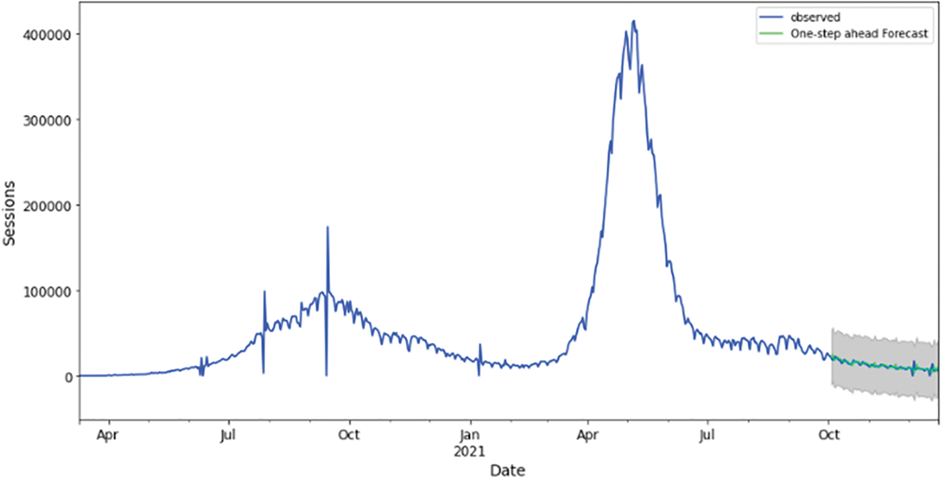
Figure 18: Training and validation datasets best fitting (best performing algorithm for India), regression trees algorithm

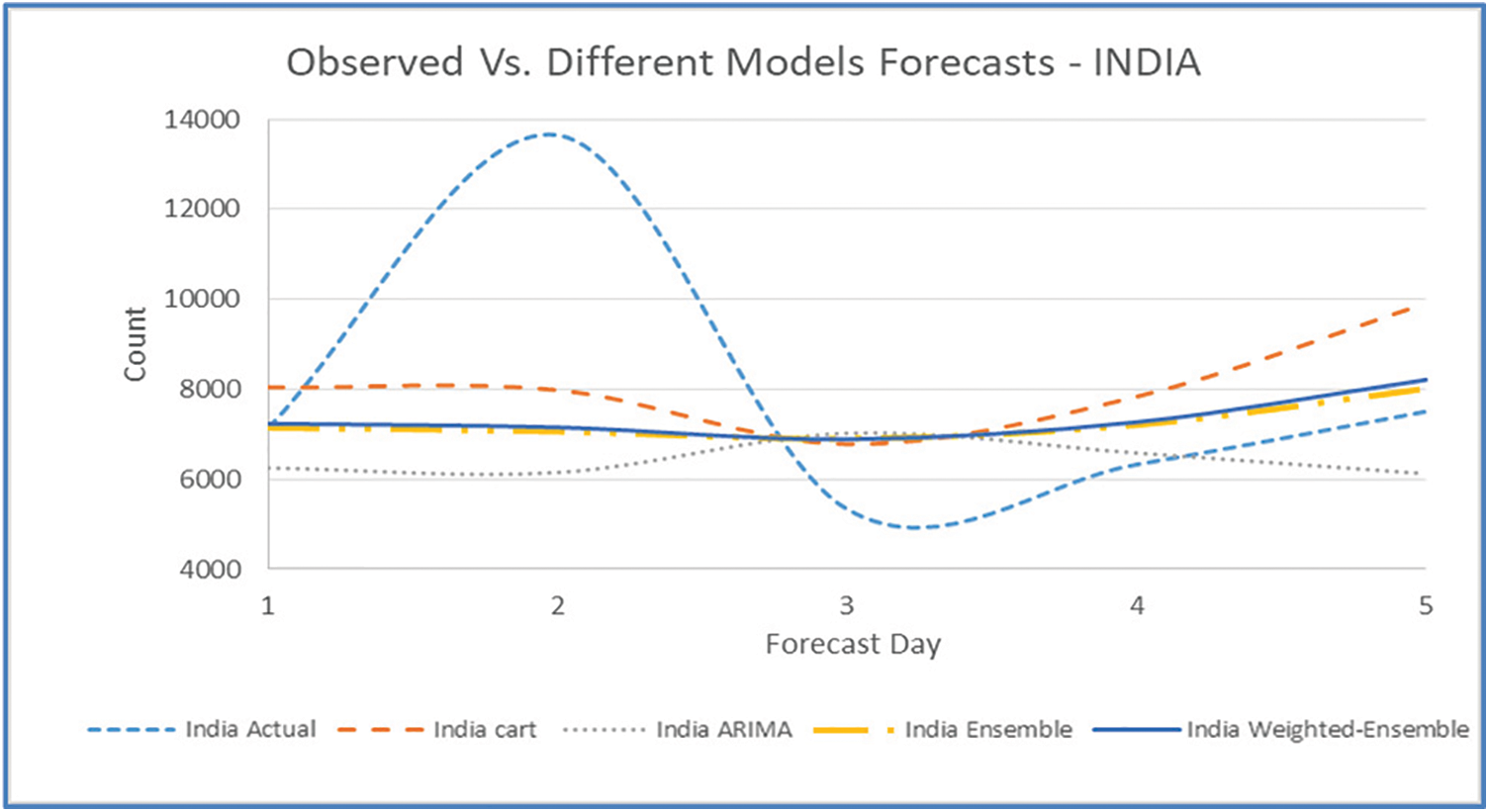
Figure 19: Five days forecast for India’s confirmed cases using the best performing ML/TS algorithms

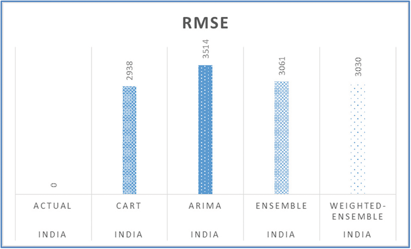
Figure 20: RMSE of five-days forecast for India’s confirmed cases using best-performing models

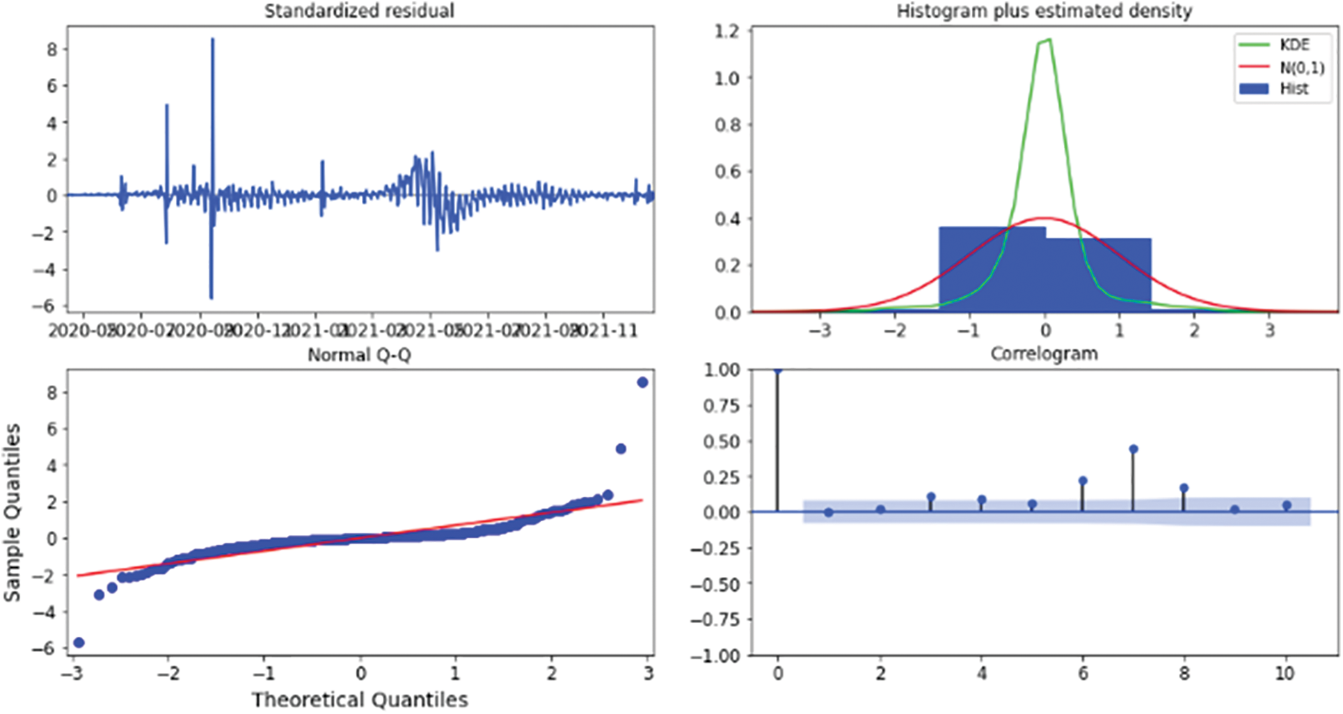
Figure 21: Results diagnostics for five-days forecast for India’s confirmed cases using the weighted ensemble algorithm

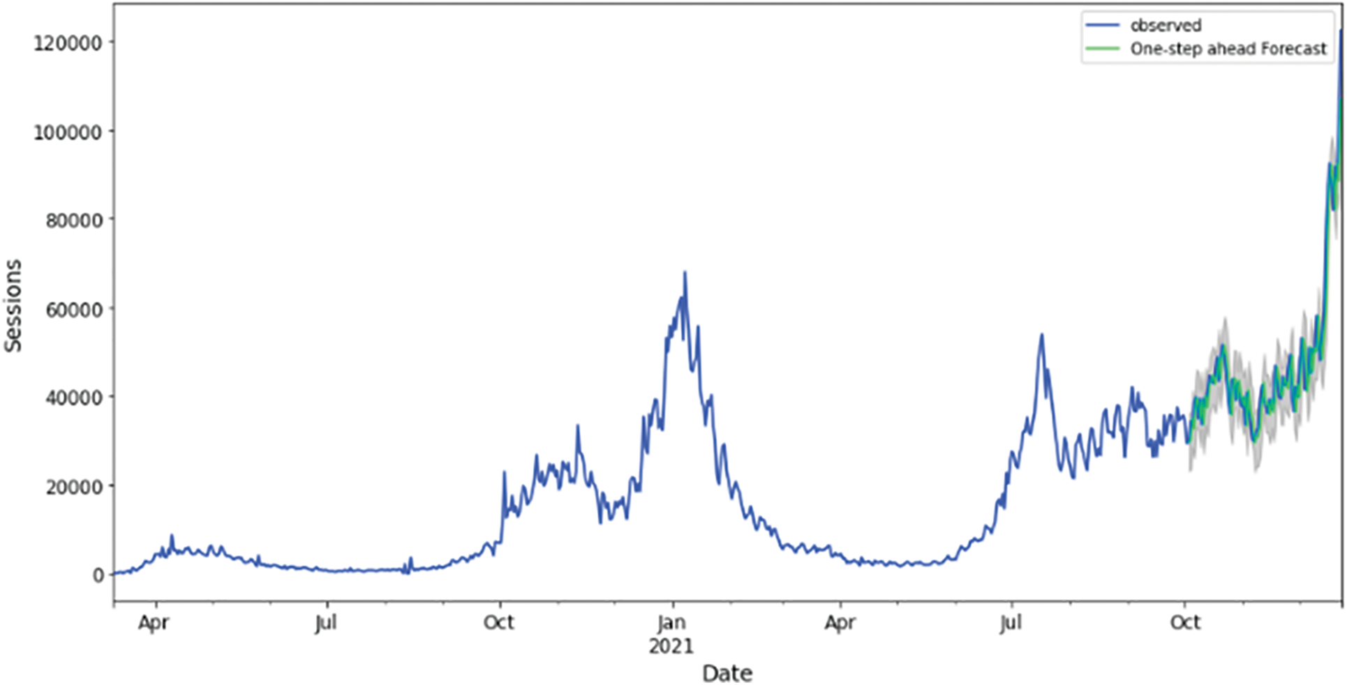
Figure 22: Training and validation datasets best fitting (best performing algorithm for UK), LLARS trees algorithm

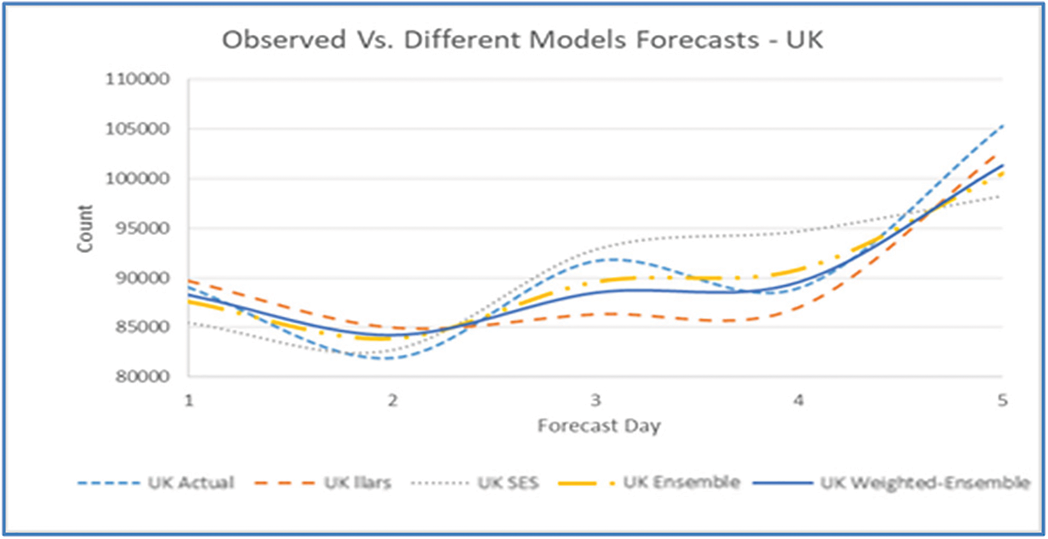
Figure 23: Five days forecast for United Kingdom’s confirmed cases using the best performing ML/TS algorithms

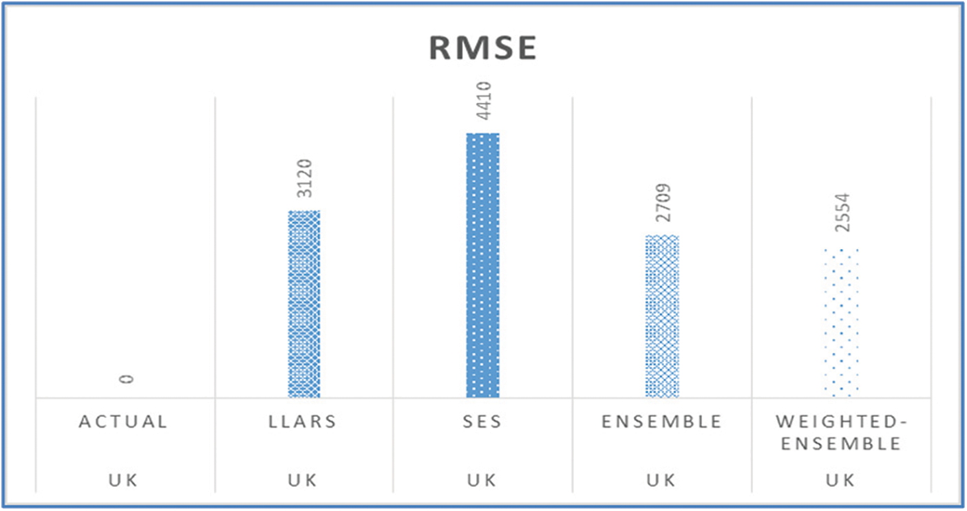
Figure 24: RMSE of the five-days forecast for United Kingdom’s confirmed cases using best-performing models

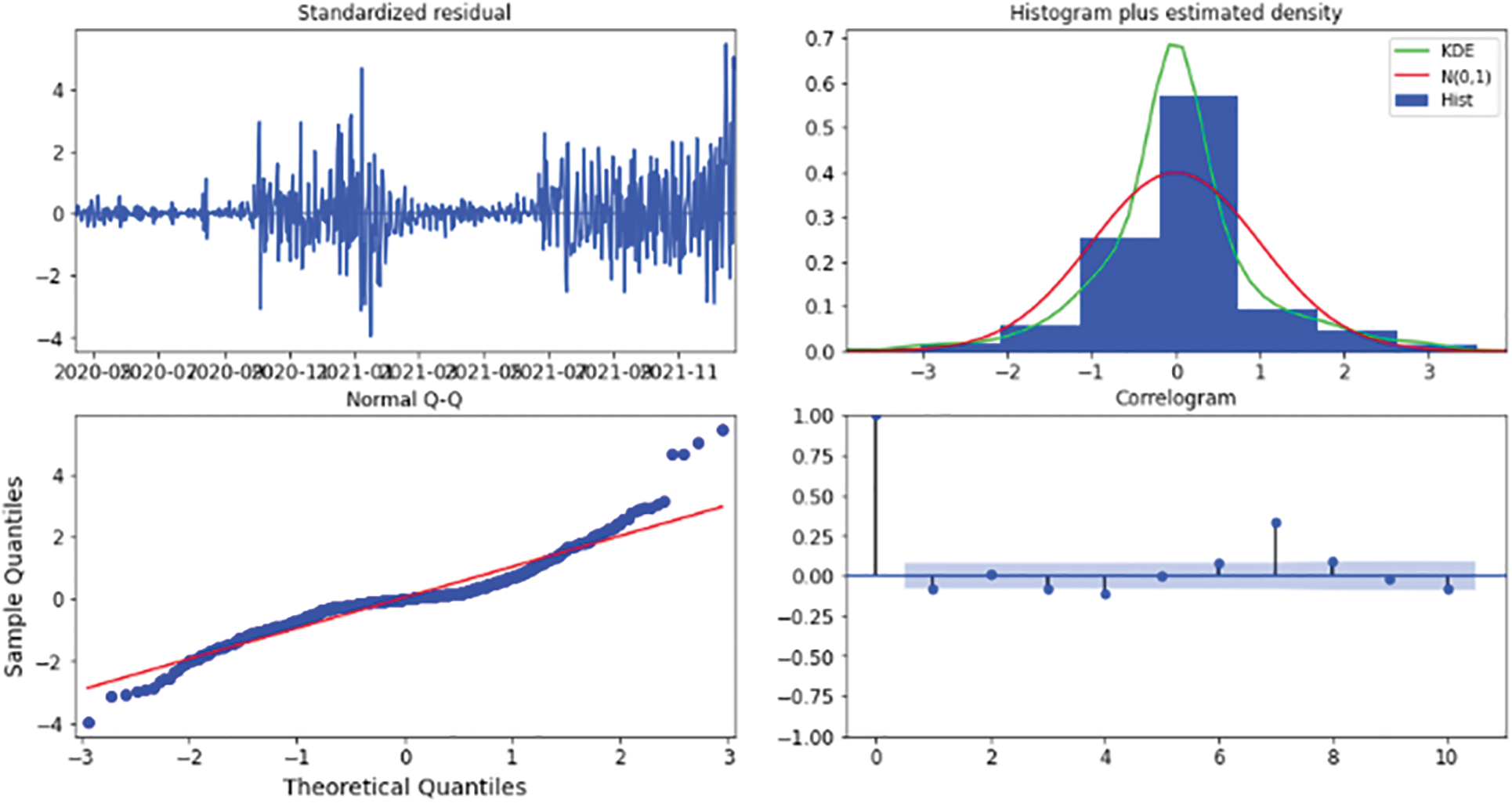
Figure 25: Results diagnostics for the five-days forecast for United Kingdom’s confirmed cases using the weighted ensemble algorithm

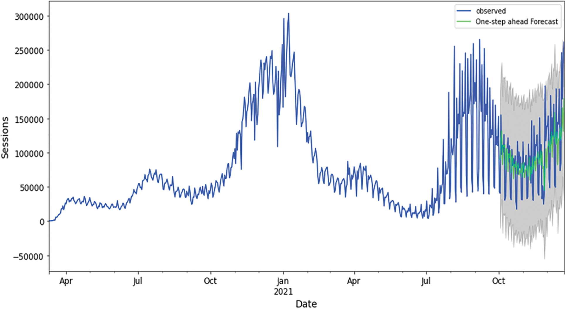
Figure 26: Training and validation datasets best fitting (best performing algorithm for USA), extra trees algorithm

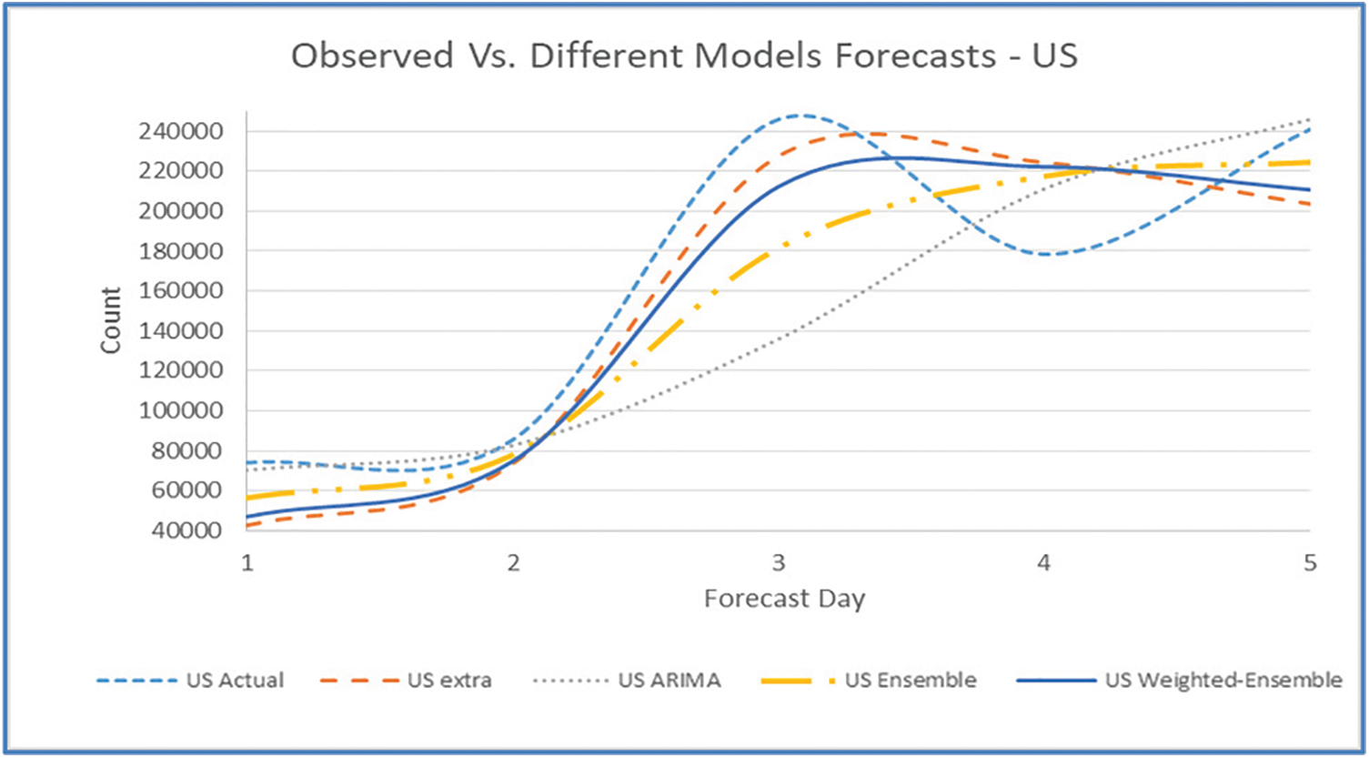
Figure 27: Five days forecast for USA’s confirmed cases using the best performing ML/TS algorithms

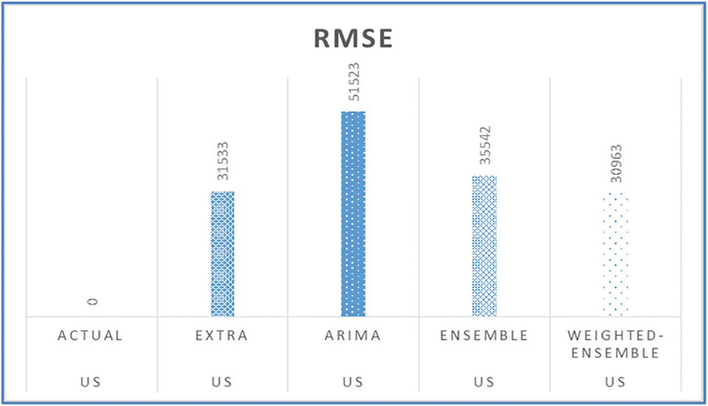
Figure 28: RMSE of the five-days forecast for USA’s confirmed cases using best-performing models

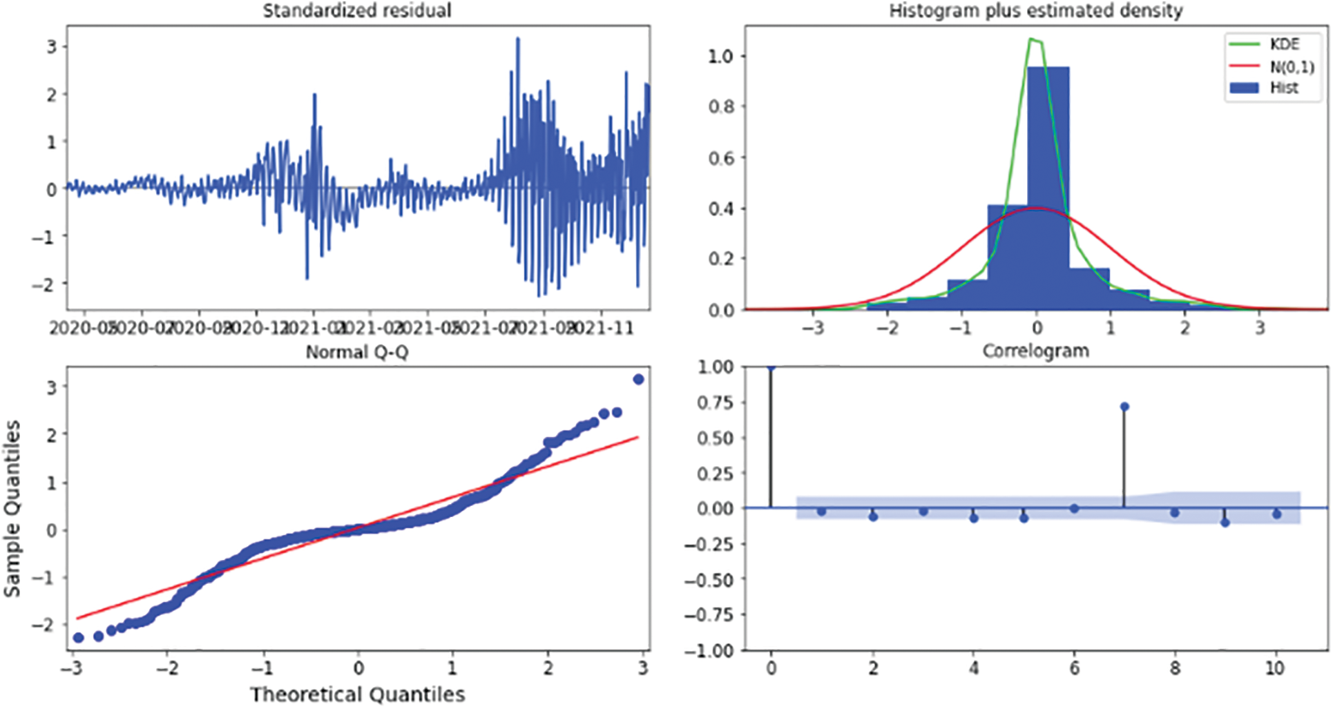
Figure 29: Results diagnostics for the five-days forecast for USA’s confirmed cases using the weighted ensemble algorithm

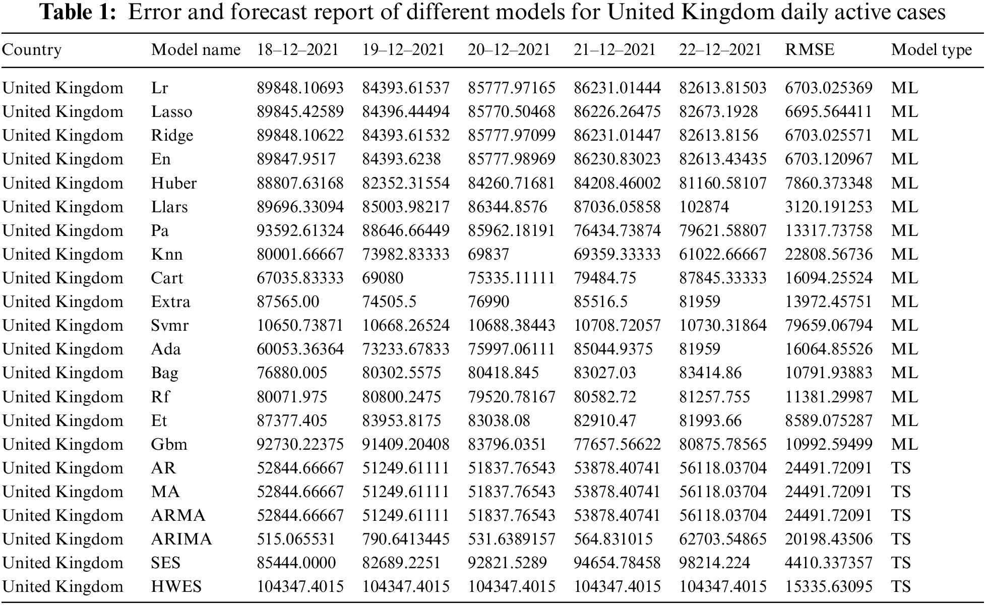
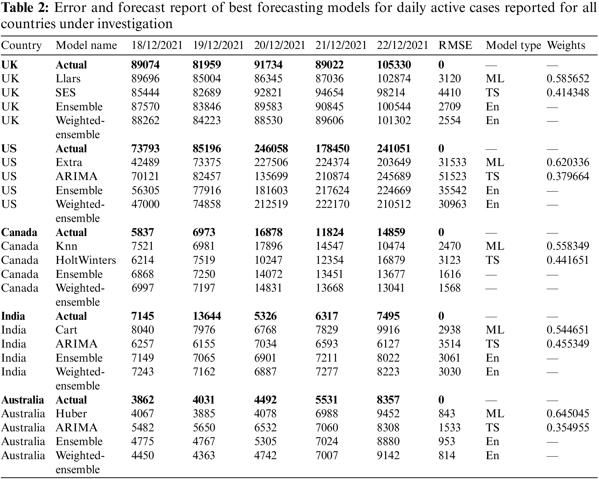
Additionally, Table 1 presents an example of the resulting forecasts of each model along with the RMSE for UK. Also, Table 2 presents the forecasts obtained from the best performing ML and statistical time series forecasting models in addition to the ensemble and weighted ensemble models. We can conclude that weighted ensemble models outperform any other model using all of these illustrations.

5  Conclusions and Future Works

In this work, we have highlighted the importance of time series forecasting models for highly accurate and reliable identification of the spread of infectious diseases. It has been proven that the forecasting time series models are very important to be utilized in identifying the spread of infectious diseases. The developed time-series regression modeling introduced in this article succeeded in collecting historical data rigorously and methodically to develop the most excellent model that can illustrate the underlying natural structure of the series in question. Thus, when tracking the evolution of an epidemic, it is vital to identify how many people will be impacted. Consequently, it is critical to tailor a suitable model to the time series. All suggested time-series models developed for forecasting infectious diseases prove their good performance when tested on different datasets. In future work, the presented work can be further well-developed to be adapted to the international society to forecast COVID-19 cases. Furthermore, we intend to propose a model for any similar pandemic outbreak forecasting.

Acknowledgement: The authors extend their appreciation to the Deputyship for Research & Innovation, Ministry of Education in Saudi Arabia for funding this research work through the project number RI-44-0525.

Funding Statement: The authors extend their appreciation to the Deputyship for Research & Innovation, Ministry of Education in Saudi Arabia for funding this research work through the project number RI-44-0525.

Conflicts of Interest: The authors declare that they have no conflicts of interest to report regarding the present study.

References

1. A. Raza, M. Rafiq, J. Awrejcewicz, N. Ahmed and M. Mohsin, “Dynamical analysis of coronavirus disease with crowding effect, and vaccination: A study of third strain,” Nonlinear Dynamics, vol. 107, no. 4, pp. 3963–3982, 2022. [Google Scholar] [PubMed]

2. N. El-Hag, G. El-Banby, A. Khalaf and N. Soliman, “An efficient CNN-based automated diagnosis framework from covid-19 ct images,” Computers, Materials & Continua, vol. 69, no. 1, pp. 1323–1341, 2021. [Google Scholar]

3. N. Ahmed, A. Elsonbaty, A. Raza, M. Rafiq W. Adel, “Numerical simulation and stability analysis of a novel reaction–diffusion COVID-19 model,” Nonlinear Dynamics, vol. 106, no. 2, pp. 1293–1310, 2021. [Google Scholar] [PubMed]

4. S. Abd El-Nabi, E. El-Rabaie, A. Ali and F. Soliman, “Efficient deep-learning-based autoencoder denoising approach for medical image diagnosis,” Computers, Materials and Continua, vol. 70, no. 3, pp. 6107–6125, 2022. [Google Scholar]

5. A. Mohamed, E. El-Rabaie, A. Ali and F. Soliman, “Automated COVID-19 detection based on single-image super-resolution and CNN models,” Computers, Materials and Continua, vol. 69, no. 3, pp. 1141–1157, 2021. [Google Scholar]

6. L. Lin, “Using artificial intelligence to detect COVID-19 and community-acquired pneumonia based on pulmonary CT: Evaluation of the diagnostic accuracy,” Radiology, vol. 296, no. 2, pp. 65–71, 2020. [Google Scholar]

7. N. Ali, C. Kaya and Z. Pamuk, “Automatic detection of coronavirus disease (covid-19) using x-ray images and deep convolutional neural networks,” Pattern Analysis and Applications, vol. 4, no. 6, pp. 1–14, 2021. [Google Scholar]

8. H. Chaolin, “Clinical features of patients infected with 2019 novel coronavirus in wuhan, China,” The Lancet, vol. 3, no. 3, pp. 497–506, 2020. [Google Scholar]

9. A. Nimai, “Infection severity detection of CoVID19 from X-rays and CT scans using artificial intelligence,” International Journal of Computer, vol. 38, no. 1, pp. 73–92, 2020. [Google Scholar]

10. W. El-Shafai, A. Algarni, G. El Banby, F. El-Samie and N. Soliman, “Classification framework for COVID-19 diagnosis based on deep CNN models,” Intelligent Automation and Soft Computing, vol. 30, no. 3, pp. 1561–1575, 2022. [Google Scholar]

11. W. Linda, Z. Lin and A. Wong, “Covid-net: A tailored deep convolutional neural network design for detection of covid-19 cases from chest x-ray images,” Scientific Reports, vol. 10, no. 1, pp. 1–12, 2020. [Google Scholar]

12. N. Soliman, S. Abd-Alhale, S. Abdulrahman and F. El-Samie, “An improved convolutional neural network model for DNA classification,” Computers, Materials and Continua, vol. 70, no. 3, pp. 5907–5927, 2022. [Google Scholar]

13. A. Nimai, “Prevention of heart problem using artificial intelligence,” International Journal of Artificial Intelligence and Applications, vol. 9, no. 2, pp. 10–19, 2018. [Google Scholar]

14. U. Ferhat and D. Korkmaz, “COVIDiagnosis-net: Deep Bayes-squeezenet based diagnosis of the coronavirus disease 2019 (COVID-19) from X-ray images,” Medical Hypotheses, vol. 14, no. 10, pp. 109–120, 2020. [Google Scholar]

15. W. El-Shafai, A. Mahmoud, E. El-Rabaie, T. Taha and F. El-Samie, “Efficient deep CNN model for COVID-19 classification,” Computers, Materials and Continua, vol. 70, no. 3, pp. 4373–4391, 2022. [Google Scholar]

16. A. Algarni, G. El Banby, F. El-Samie and N. Soliman, “An efficient CNN-based hybrid classification and segmentation approach for COVID-19 detection,” Computers, Materials and Continua, vol. 70, no. 2, pp. 4393–4410, 2022. [Google Scholar]

17. W. Wenling, “Detection of SARS-CoV-2 in different types of clinical specimens,” Jama, vol. 3, no. 3, pp. 1843–1844, 2020. [Google Scholar]

18. O. Tulin, “Automated detection of COVID-19 cases using deep neural networks with X-ray images,” Computers in Biology and Medicine, vol. 12, no. 1, pp. 103–114, 2020. [Google Scholar]

19. W. Jon, “Steps toward architecture-independent image processing,” Computer, vol. 25, no. 2, pp. 21–31, 1992. [Google Scholar]

20. F. Abd El-Samie, “Extensive COVID-19 X-ray and CT chest images dataset,” Mendeley Data, v3. 2020. http://doi.org/10.17632/8h65ywd2jr.3 [Google Scholar] [CrossRef]

21. E. Gecili, A. Ziady and R. Szczesniak, “Forecasting COVID-19 confirmed cases, deaths and recoveries: Revisiting established time-series modeling through novel applications for the USA and Italy,” PLoS ONE, vol. 16, no. 3, pp. 1–23, 2021. [Google Scholar]

22. F. Shi, J. Wang, J. Shi, Z. Wu and D. Shen, “Review of artificial intelligence techniques in imaging data acquisition, segmentation, and diagnosis for COVID-19,” IEEE Reviews in Biomedical Engineering, vol. 14, no. 5, pp. 4–15, 2021. [Google Scholar] [PubMed]

23. L. Harper, N. Kalfa, G. Beckers, M. Kaefer and A. Nieuwhof-Leppink, “The impact of COVID-19 on research,” Journal of Pediatric Urology, vol. 16, no. 5, pp. 715–716, 2020. [Google Scholar] [PubMed]

24. K. Prem, Y. Liu, T. Russell, A. Kucharski and P. Klepac, “The effect of control strategies to reduce social mixing on outcomes of the COVID-19 epidemic in wuhan, China: A modelling study,” The Lancet Public Health, vol. 5, no. 5, pp. 261–270, 2020. [Google Scholar]

25. W. Yang, D. Zhang, L. Peng, C. Zhuge and L. Hong, “Rational evaluation of various epidemic models based on the COVID-19 data of China,” Epidemics, vol. 3, no. 7, pp. 100–121, 2021. [Google Scholar]

26. Z. Wang, Q. Wu, S. Feng, Y. Zhao and C. Tao, “Identification of four prognostic LncRNAs for survival prediction of patients with hepatocellular carcinoma,” PeerJ, vol. 5, no. 7, pp. 35–45, 2017. [Google Scholar]

27. M. Wieczorek, J. Siłka and M. Woźniak, “Neural network powered COVID-19 spread forecasting model,” Chaos, Solitons & Fractals, vol. 14, no. 10, pp. 110–123, 2020. [Google Scholar]

28. E. Maddah and B. Borhan, “Use of a smartphone thermometer to monitor thermal conductivity changes in diabetic foot ulcers: A pilot study,” Journal of Wound Care, vol. 2, no. 9, pp. 61–66, 2020. [Google Scholar]

29. R. Sujath, J. Chatterjee and A. Hassanien, “A machine learning forecasting model for COVID-19 pandemic in India,” Stochastic Environmental Research and Risk Assessment, vol. 34, no. 7, pp. 959–972, 2020. [Google Scholar] [PubMed]

30. A. Zeroual, F. Harrou, A. Dairi and Y. Sun, “Deep learning methods for forecasting COVID-19 time-series data: A comparative study,” Chaos, Solitons & Fractals, vol. 140, no. 11, pp. 111–121, 2020. [Google Scholar]

31. K. Pokkuluri and S. Nedunuri, “A novel cellular automata classifier for covid-19 prediction,” Journal of Health Sciences, vol. 10, no. 1, pp. 34–38, 2020. [Google Scholar]

32. A. Payedimarri, D. Concina, L. Portinale and M. Panella, “Prediction models for public health containment measures on COVID-19 using artificial intelligence and machine learning: A systematic review,” International Journal of Environmental Research and Public Health, vol. 18, no. 9, pp. 44–66, 2021. [Google Scholar]