Deep Autoencoder-Based Hybrid Network for Building Energy Consumption Forecasting

1  Introduction

The increasing population on a global scale, advancements in economics, and industrialization have significantly influenced international PC and environmental concerns [1]. The majority of people spend their waking hours inside buildings, increasing energy consumption for building activities, a result of which is an increase in the total amount of energy consumed by the building. Accordingly, the contribution of residential buildings to greenhouse gas emissions and PC globally is 38% and 39%, respectively. According to research findings, electricity consumption management has become a vital study topic as a result of insufficient supply of energy, emissions of greenhouse gases, energy demand worldwide, and a lack of clean and sustainable energy systems [2]. Forecasting loads play a crucial part in guaranteeing the reliability and safety of energy systems. Improved power productivity of residential and commercial buildings can be achieved by establishing robust and accurate load forecasting models. It has been very helpful for both residential and commercial building customers and suppliers to develop load forecasting solutions [3]. These solutions allow them to make better decisions, reduce costs, and avoid any possible power grid issues.

In smart homes, energy consumption predictions, like load forecasting, have become an increasingly important part of energy management systems [4]. According to the timeframe of the forecast, there are three main categories of power prediction range. Short-term PC prediction duration ranges from one hour to one week. Similarly, the medium-term prediction range can be in weeks and cover a period of moderate length. Long-term forecasting refers to forecasting over a long timeframe, often months or years [5]. However, due to the advancement in the technologies of smart meters and the Internet of Things (IoT), a large amount of PC and weather data is produced and stored [6]. The data can be used for modeling load forecasting data-driven Artificial Intelligence (AI) algorithms. The short-term PC curve provides information about the correlation between data and their corresponding working day or holiday. Various factors that are uncontrollable and affect PC patterns. PC is a time series and depends on various conditions such as consumer behavior and weather, which make its prediction more challenging [7]. Additionally, automatic management of building energy systems, renewable energy systems, power storage, and electrically powered equipment is made possible through short-term load forecasting [8]. Researchers must take these challenges into account when investigating short-term PC prediction in various sectors.

Nowadays, a large amount of PC data is available due to the advancement in the smart meter and IoT technologies due to which, it has been possible to explore data-driven methods instead of physics-driven techniques [9]. Several statistical and ML approaches have been investigated in the past to predict PC including Auto-Regressive Integrated Moving Average (ARIMA) [10], fuzzy models [11], linear and non-linear Regressors [12], Artificial Neural Networks (ANN) [13], and ensemble techniques [14]. Traditional statistical and ML techniques are unable and fail to learn the nonlinear PC patterns of commercial and residential buildings. However, there are several other research domains such as computer vision [15] and bioinformatics [16] where Deep Learning (DL) networks are also investigated and proved very effective compared to the traditional approaches. In the case of large datasets, DL models such as deep Neural Networks (NN), CNN, and Recurrent Neural Networks (RNN) obtain remarkable performance. Although DL models are a well-established concept in different domains, however, they are not explored in short-term load forecasting as in other research areas. The strengths of DL approaches are demonstrated in former studies by exposing CNNs, and RNNs to significant performance improvements compared to conventional approaches for PC prediction. As a result, we are motivated to apply DL-based hybrid network in short-term load prediction. Following are some important research gaps that remain unexplored or partially explored in the current literature on PC forecasting:

•   Due to rising electricity consumption, a shortage of energy supplies, and hazardous pollutants, there is a research gap in green energy research, which has raised the need for energy management research. Forecasting residential and commercial building demand is crucial for power management, smart grid scheduling, and making wise choices about building energy.

•   Data-driven methodologies have made significant advancements, but little research has been done on the use of streaming and temporal data in forecasting buildings’ energy demand.

•   Recent studies have uncovered serious issues due to variations in location, size, building type, people activities, and energy consumption patterns, the peak load of buildings can vary significantly.

•   PC forecasting approaches have a significant drawback in that they are often created for houses in comparable surroundings and building types. As a result, these techniques might not be useful for anticipating energy use in buildings that are diverse and spread out throughout different regions.

•   PC data is collected via different sensors and meters, which have various anomalies and cannot be used for AI model training directly.

To improve residential and commercial short-term load prediction, this paper addresses the discussed research gaps with the following main contributions:

•   In this study, an intelligent hybrid network is proposed, which is referred to as data-driven and dependent on the DL approach for short-term PC prediction. The network is suitable to clean the raw data and predict the PC of different types of buildings in various conditions and locations.

•   The front end of the proposed network consists of a one-dimensional CNN-based deep AE. The AE is first trained on different commercial and residential buildings’ PC data, to learn the more compressed and efficient features. After obtaining remarkable results in reconstruction by the AE, its encoder part is used to extract the representative spatial features from PC datasets and passed them to the online sequential ELM.

•   The back end of our network uses online sequential ELM for the learning of the compressed features, which are extracted by the encoder. Since commercial and residential PC data is a time series and depend on different environmental, consumers, and weather conditions. Additionally, for streaming data, online sequential ELM provides a fast rate of learning as well as satisfactory generalization results.

•   To demonstrate the effectiveness of the proposed network in different types of environments and buildings, we use two buildings’ PC datasets from different places. In comparison, the experiment results demonstrate that our model obtains less error when compared to the SOTA techniques.

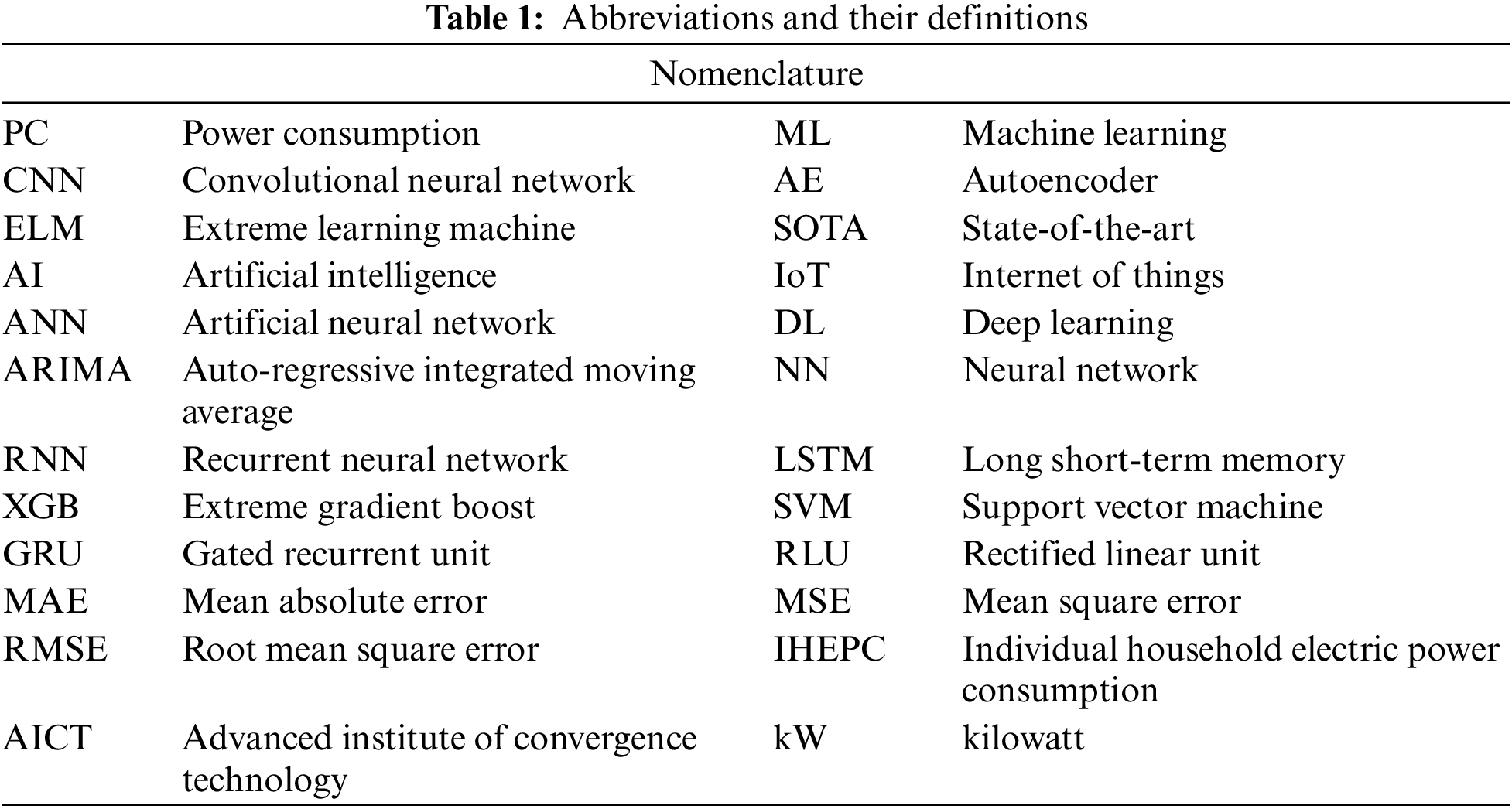
Further study is organized as follows: The proposed model and its related components are provided in Section 3 after a detailed analysis of the types of recent studies that examined PC prediction in Section 2. The experimental results are presented in Section 4 along with a detailed discussion and analysis of them, while the overall conclusions are presented in Section 5. All the abbreviations and their definitions are mentioned in Table 1.

2  Related Work

There are several uses for AI across numerous domains such as face recognition [17], edge detection [18], ovarian [19] and osteosarcoma [20] cancer classification, network meddling detection [21], stock [22] and its closing price forecasting [23]. Similarly, different approaches in the literature have been used for various types of consumption forecasting. PC forecasting plays an important role in a power management system. The detailed literature review is discussed as follows.

2.1 Traditional Machine Learning Approaches

To overcome the main challenges faced by the physics-driven methods, ML algorithms have been explored for load prediction. For instance, Abiyev et al. [24] introduced a novel approach based on fuzzy set theory for the prediction of energy performance. They used type-2 fuzzy wavelet NN for two types of issues where in the first problem cooling and heating load is predicted while in the second step, the PC in the residential buildings is forecasted. Next, Wang et al. [25] forecasted the thermal load of buildings using twelves ML and DL models. In their comparison, they concluded that for the short-term PC prediction, the performance of the Long Short-Term Memory (LSTM) network was remarkable while Extreme Gradient Boost (XGB) performed well for long-term forecasting. In addition, Li [26] conducted experiments for PC forecasting in smart grid management where the used model was ANN. Further, Dietrich et al. [27] developed ANN for the PC of machine tools in a factory. Their study found that machine tools PC prediction can play an important role in power management and cost reduction of power in industries. Liu et al. [28] incorporated Holt-Winters and ELM and forecasted the PC of a residential building. They preprocessed the consumption data and divided it into various components such as linear and nonlinear where Holt-Winters was used to learn the linear components while ELM is employed for the nonlinear components of the original data. Dai et al. [29] conducted experiments on ML algorithms by exploring Support Vector Machine (SVM) and predicted PC. They also investigated feature selection approaches and different parameters of SVM, and chose those on which the performance is notable.

2.2 Deep Learning Approaches

In AI, data mining refers to methods that use input information to capture and extract hidden intrinsic characteristics and high-level structures. The main limitations of traditional ML approaches can be addressed using DL models. In this context, Park et al. [30] used a deep Q-Network procedure, which was a reinforcement technique to select the same days in the consumption data, and then ANN was trained for PC prediction. Next, Nam et al. [31] compared different algorithms for power generation and consumption considering different scenarios in South Korea. They experimentally proved that the performance of the Gated Recurrent Unit (GRU) was best compared to the other forecasting models. Liu et al. [32] conducted a comparative study of three different types of techniques for load forecasting that were classical regression, traditional time series techniques such as ARIMA, and DL models such as CNN. Further, they studied the effect of feature selection and encoding techniques for the best model selection. Chitalia et al. [33] compared nine DL models and clustering algorithms for five different commercial building load forecasting datasets. Yin et al. [34] proposed a novel approach based on temporal convolutional NN for short-term PC prediction. Their technique has the ability to learn the time series and nonlinear characteristics from the cleaned PC data. Imani et al. [35] proposed LSTM for residential load prediction that employed collaborative and wavelet representation transforms. Xu et al. [36] illustrated an ensemble approach for short-term PC forecasting where the algorithm had residual connections that were based on fully connected layers. He et al. [37] proposed a one-dimensional CNN for the consumption prediction of machine tools. They used two machine tools data including grinding and milling machines and showed that their proposed approach outperformed the other baseline methods.

There are also several networks where multiple techniques are integrated to design data-driven approaches. These mechanisms are also known as hybrid networks. For instance, Li et al. [38] introduced a novel approach that integrated multivariable linear regression and LSTM for short-term PC prediction. In their approach, the PC data were decomposed where multivariable linear regression was trained on linear components while LSTM was nonlinear, and both models’ output was combined for final load forecasting. Next, Heydari et al. [39] developed a mixed model for the consumption data that predict short-term PC and price. Further, Wang et al. [40] investigated industrial consumption data and developed a hybrid model that combined temporal CNN for hidden feature learning and an ensemble learning algorithm for short-term PC prediction. He et al. [41] forecasted short-term PC using a probability density and quantile regression approach. Hafeez et al. [42] proposed an approach that incorporated data preprocessing, feature selection, and the Boltzmann machine, which was a DL model for PC forecasting. Kong et al. [43] predicted PC for a short-term interval using the approach based on the correction and forecasting of the errors. Somu et al. [44] developed a network for building PC forecasting based on LSTM. Further in their study sine cosine optimization algorithm was employed to improve the prediction performance. Cascone et al. [45] proposed a two phases network based on LSTM and convolutional LSTM for residential load consumption forecasting. The main types of PC prediction approaches and their limitation are given in Table 2.

3  Methodology

The steps involved in the proposed framework are explained in this section. The main steps are data preprocessing, model training, and testing as shown in Fig. 1.

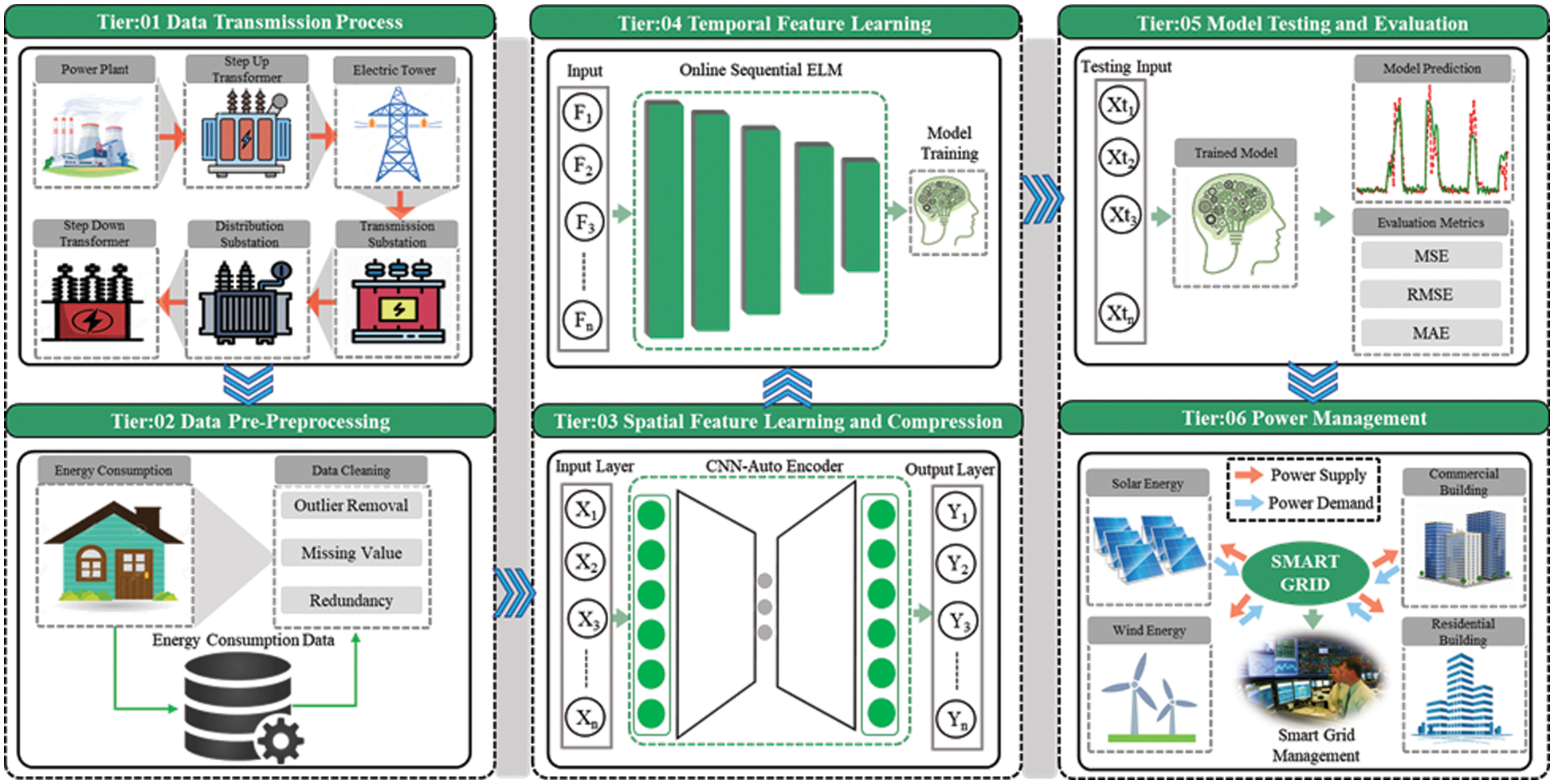
Figure 1: The working flow of the proposed framework consists of various steps. First, the consumption data of commercial and residential buildings are collected, and then preprocessing step is applied to make the raw data clean and suitable for model training. Next, AE is trained and used to extract the compressed spatial patterns from the data, which are then provided to the online sequential ELM for short-term load forecasting. Finally, the model predictions are visualized and analyzed, which can be used for building or grid energy management

3.1 Data Acquisition and Preprocessing

Data-driven methods depend on the input data and its quality. However, the consumption data of commercial and residential buildings may contain a lot of abnormalities. Hence, PC data is measured through smart meters, which are affected by several environmental factors. The data obtains from these smart meters is not perfect and has not good quality due to which it cannot be used directly to train the data-driven ML and DL algorithms. To obtain remarkable and high results from the ML and DL networks, the raw data of smart meters should be preprocessed. PC data is a time series and for that type of data, there are several preprocessing approaches, which include cleaning, normalizing, and smoothing are some of the most common. One import issue in PC data is missing attributes and outlier values, which are solved with the help of the cleaning process [56]. In the proposed framework first, the missing and outliers values are detected and then replaced with the mean value. Similarly, Savitzky-Golay filters are used as a smoothing method in the study to make the input data more efficient for the training process. Furthermore, the second issue in the PC data is a different scale. There are different attributes in the consumption data that have different scales. Since it is proved in previous studies that DL networks perform well with the data having the same range. Therefore, in this study, we also convert the PC data to a specific range using the normalization approach. Eqs. (1) and (2) are used to normalize the input features and output values, respectively. These equations include Ik as input data, Ok as output data, Imin, Imax and Omin, Omax are the smallest and largest values of Ik and Ok, respectively, while I^k and O^k are input and output normalized data.

I^k=Ik−IminImax−Imin(1)

O^k=Ok−OminOmax−Omin(2)

3.2 Proposed Hybrid Model

This section provides details about the various components of the proposed hybrid model. There are two main components in the model that include CNN-based deep AE and online sequential ELM. The proposed model has several advantages that distinguish it from the other models. The AE component of the model can learn the local features, perform a non-linear transformation, compress the power data, and have unsupervised learning ability. The AE is important for the effective and efficient learning of the complex feature extraction from the PC time series data. Due to this, manual feature engineering and data labeling are reduced. Similarly, the other component of the proposed hybrid model is online sequential ELM, which is very effective for the analysis of PC data. It is very useful due to the quick training, more general performance, adaptability to the changes in the environment, and the ability of online learning. These components are explained in the following subsections.

3.2.1 CNN-Based Autoencoder

Univariate and multivariate time series data are often used for forecasting or classification problems. Among the uses may be the classification of activity from sensor data, the prediction of weather in the future, or analyzing the voice data for different purposes. However, time series are often accompanied by a considerable amount of noise. An example of this is the fact that sensor readings are notoriously noisier than other forms of data, and they often contain patterns that are not related to the actual data such as in the case of load consumption in houses. The application of smoothing techniques in time series analysis has traditionally been a part of the analysis process. A moving average can be applied to smooth a time series before applying a forecasting or classification technique. Similarly, based on the domain knowledge weighted moving average technique can also be utilized. But not in the case of big data in smart grids and homes, it is a very challenging task to automatically calculate the weights for smoothing and to determine that the chosen parameters are good for leveling the data [57].

To learn smoothing parameters, a network architecture is needed that is based on CNNs. There are two main layers in a CNN: the first is a convolutional layer and the second is a pooling layer where both accomplish smoothing functions [58]. When a CNN-based loss is optimized, the smoothing parameters are also optimized because these two layers are part of a prediction function. Time series forecasting or classification then takes place in the later layers using the smoothed raw data obtained from the above two layers. Convolutional layers receive a fixed-length sub-sequence of full-time series data as input from the input layer. Input is first smoothed by the convolutional operation and then by pooling layers. With the Rectified Linear Unit (RLU) layer, the smoothed sub-sequence from the two layers is transformed using an RLU, which is a nonlinear activation, and the output of it is a vector-valued result that is then plugged into a different activation function to produce class probabilities, or a continuous-valued response depending on the type of activation function used. The concept of a convolution operation can be described as the weighted sum of memories or echoes. A pooling strategy involves chunking a vector into nonoverlapping equal-sized groups, then calculating the summary statistic for each group. In addition to smoothing out local dynamics, max pooling is commonly used with image data, average or mean pooling, and min pooling. Putting non-linearity on the smoothed vector obtained from the convolutional and pooling layers prepares it for the final output layers. After two layers of smoothing and one layer of non-linear transformation are applied to the original data, in the final output layer, an activation function is applied to a weighted sum of that representation to generate output data of the relevant type based on our choice of the activation function. It could be used for class probabilities or continuous responses depending on the problem domain. In this study, we consider one-dimensional CNN due to its high and efficient performance in different domains for the proposed AE.

AEs are unsupervised learning techniques that utilize ANNs to learn representations from the input data. The ANN architecture in AE is constructed where a bottleneck is created in the network that forces the original input sequence to be compressed into compacted knowledge [59]. The compressed representation is then converted to the clean original input. This compression and subsequent reconstruction are difficult if the input features are independent. Despite this, if the input features may have some structure, i.e., correlations between them, that structure can be learned and leveraged to force them through the network’s bottleneck. An unlabeled dataset is changed for AE to a supervised problem where the network task is to reconstruct the actual data. To train this network, the restoration loss is minimized that measures the variance between the actual data and the subsequent reconstruction. There is a bottleneck in AE network design, without which input values would simply be memorized as they are passed through the model. When there is a bottleneck in the AE network, the amount of information that can traverse it is restricted, which results in the input data having to be compressed in a learned manner. AEs play an important role to balance the two main factors. It is sensitive enough to the inputs to build accurate reconstructions. Training data should not become memorized or overfitted by the model due to its sensitivity to inputs. By preserving only, the variations in the data needed for reconstruction, the model is not preserving redundant inputs. The most common way to do so is to construct a loss function that has two terms, one of which encourages sensitivity to the inputs, i.e., reconstruction loss, and another which discourages memorization and overfitting, i.e., regularization. A scaling parameter is usually added before the regularization term to adjust the trade-off between the two objectives. Motivated by the significant results of the CNN and AEs in different fields, in this study we develop an AE, which is made from the one-dimensional CNN, as visualized in Fig. 2a. First, the PC data of commercial and residential buildings is preprocessed and transformed into a supervised learning form. Next, the AE architecture is trained on that data until it obtained satisfactory results for reconstructing the output. Finally, the encoder part of the trained AE is removed and used as a compressed and representative features extractor from time series PC data. These extracted features are used for training the online sequential ELM for final short-term PC forecasting in different sectors.

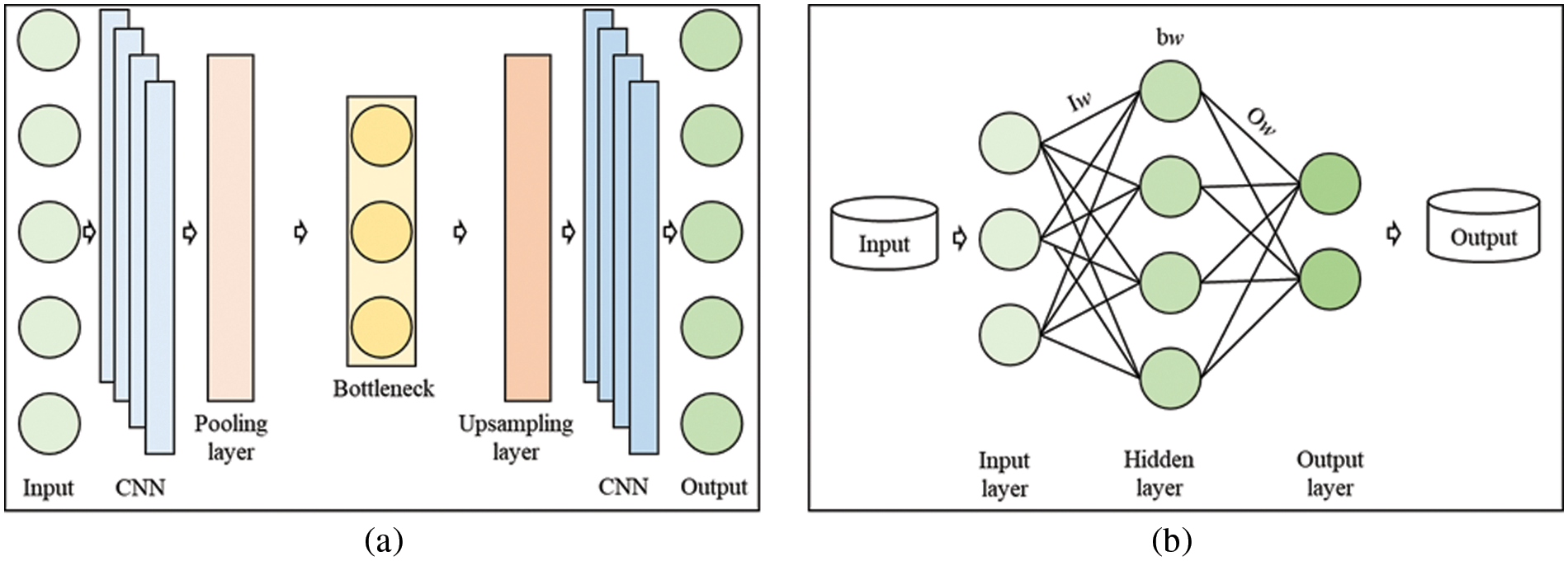
Figure 2: (a) Structure of Autoencoder for the compressed features extraction that mainly consists of CNN and upsampling layers, (b) Basic overview of the extreme learning machine architecture

3.2.2 Online Sequential Extreme Learning Machine

Single-layer ANN, which is also known as perceptron is a type of feedforward NNs. A single-layer perceptron accepts data through the input layer, hidden layer neurons perform the weighted sum operation, and the output layers provide the prediction according to the problem. There are several neurons in the hidden layer that conduct the weighted addition of the input data and corresponding weights. If the output of a neuron is greater than some threshold value, its value is considered 1 otherwise 0 in case of the neuron output is less than the threshold. Simple feedforward NN obtains significant performance in classification and regression-related tasks but these networks are slow, affected by vanishing gradient issues, and not suitable for time series sequential problems such as load consumption data. To handle the mentioned issues ELM was introduced, which is faster and provides more generalized results compared to the traditional feedforward ANNs [60]. ELMs belong to the category of feedforward NNs and can be employed for different tasks such as compression, classification, clustering, and regression. ELM can have a different number of hidden layers but the difference from traditional ANNs is that its hidden layers’ weights are not changed. These weights are assigned randomly to the hidden layers or inherited from forerunners and are not updated again. ELMs are faster in learning than the traditional feedforward ANNs because these network hidden layers’ weights are commonly obtained in a single step. Furthermore, ELMs can yield more generalized results compared to the traditional backpropagation NNs.

Feedforward NNs can be trained in a quicker way using ELMs. There are three layers in a simple ELM that include input, output, and hidden layers as shown above in Fig. 2b. In the input layer, there is no calculation involved while the output layer also does not use bias and transformation functions but performs linear operations. In this technique, random weights for the input layer and biases are selected while these are not updated again. In the ELM method, the weights of the output do not depend on the weights of the input because fixed weights are used in the input. Since in backpropagation the input weights are not fixed, therefore ELM does not need iteration for the solution. In the case of liner output the computation for the output is also very fast. By assigning the weights of the input layer randomly, the liner output layer solution properties can be generalized because the features of the hidden layer are correlated weakly. Linear system solution has a strong relation to the input. As a result, decent generalized results and trivial norms for a solution can be obtained using the random hidden layer. Because the features of the hidden layer in this case are weakly correlated. ELM can be described in Eq. (3), where iϵ[1,M], fiϵRd, M is a set of different training data samples (fi, ti), tiϵRc , and N is the number of hidden layer neurons. Similarly, ϕ is the activation function, Ij, bj, and Oj are input weights, biases, and output weights respectively. Model predicted output pN, target output ti, and its input fi the relation can be represented using Eq. (4), where ϵ is for the noise.

pN=∑j=1NOjϕ(Ijfi+bj), iϵ[1,M](3)

pN=∑j=1NOjϕ(Ijfi+bj)=ti+ϵi, iϵ[1,M](4)

The type and nature of data in the real world are different such as images, time series, text, and voice data. PC data is a time series and it varies and increases with time where the complete data is impossible to access or use for modeling and training. Therefore, instead of using the traditional ELM model, there should be changes in the network that learns the dynamic changes in sequential load consumption data. The data increases with time, thus we have to train the ELM again and again as new data is included in the basic dataset. However, the newly added data is small in the portion, and training the network again and on all datasets is an inappropriate and inefficient way. To handle these issues, in this study, we use online sequential ELM, which can be trained efficiently on the PC data. Online sequential ELM solved the issue of training again and again on the complete dataset using the sequential technique [61]. In addition, it can change the parameters according to the new data samples. In the proposed framework, PC data of commercial and residential buildings is provided to the CNN-based AE, which employed an encoder part to extract the representative and compressed features from the input sequences. Next, these compressed and efficient features are fed to the online sequential ELM that learns temporal and dynamic relation and forecast the short-term PC for different buildings.

4  Experiments and Discussion

This section provides detail about the implementation and evaluation criteria of the proposed model, datasets, ablation studies, and comparison with SOTA.

4.1 Implementation Setup and Evaluation Metrics

The proposed model consists of two networks that include CNN-based AE and online sequential ELM. The AE is implemented in the famous DL library known as Keras with the 2.4.0 version while it uses TensorFlow version 2.4.0 as a backend. For the implementation of the online sequential ELM Pyoselm library is utilized. Similarly, the installed Python version is 3.8.5, the operating system is Windows 10, 48.0 gigabytes of random access memory while the computer system has a GeForce RTX 3090 graphics processing unit of the NVIDIA and AMD Ryzen 9 3900X 12-Core processor. To train the AE model Adam is selected as an optimizer with a learning rate of 0.001, 64 batch size, and 100 epochs. Furthermore, the encoder architecture consists of three CNN layers each follows by a max pooling layer with filter size 7. Similarly, the decoder contains three layers of transposed CNN layers to upsample the features with kernel size 7. All these hyperparameters are tuned using the Grid search algorithm, which is very efficient and checks all the possible combinations. In this study, the predictions of all models used in the ablation studies are evaluated using five main evaluation metrics given in Eqs. (5)–(9). These error metrics are Mean Square Error (MSE), Mean Absolute Error (MAE), Root Mean Square Error (RMSE), R-squared (R2), and Adjusted R-squared (AR2). In these equations Gi is ground truth, Fi is the forecasted result, G¯ is the mean of actual values, K is a number of independent features while T represents the total samples for the evaluation.

MSE=1T∑i=1T(Gi−Fi)2(5)

MAE=1T∑i=1T|Gi−Fi|(6)

RMSE=1T∑i=1T(Gi−Fi)2(7)

R2=1−∑(Gi−Fi)2∑(Gi−G¯)2(8)

AR2=1−[(T−1T−K−1)∗(1−R2)](9)

4.2 Power Consumption Datasets

In this study, our goal is to develop a model that can forecast PC in different environments and sectors without affecting by various environmental issues such as consumer behavior and location. Considering this we use two real-world PC datasets one from a residential building named Individual Household Electric Power Consumption (IHEPC) [62] while the second one is from a commercial building known as Advanced Institute of Convergence Technology (AICT) for evaluating the proposed method. The IHEPC dataset recorded the total PC data of a residential building in one-minute resolution where the home is located in Sceaus, France. Furthermore, this data also records the values for the other parameters such as appliances, reactive power, intensity, and voltage. The total dataset is recorded for the forty-eight months starting from December 2006 and ending in November 2010. Furthermore, the IHEPC dataset has null values in the form of missing data. Similarly, the AICT is a PC dataset of a commercial building located in South Korea and is similar to the IHEPC dataset but there are some differences also. For instance, the data is recorded in the AICT dataset in fifteen-minute resolution while in IHEPC data it is stored in one-minute resolution. Further, in AICT data two sub-meter data are available but in IHEPC three sub-meter data are recorded. Similarly, the data recording duration and places are also different such as the AICT data recorded from January 2016 to December 2018. In this study, we consider the hourly resolution of both datasets, and the main attribute, which is the actual load consumption is utilized for short-term forecasting. The samples of both consumption datasets are visualized in Fig. 3 using hourly resolution while their summary is given in Table 3.

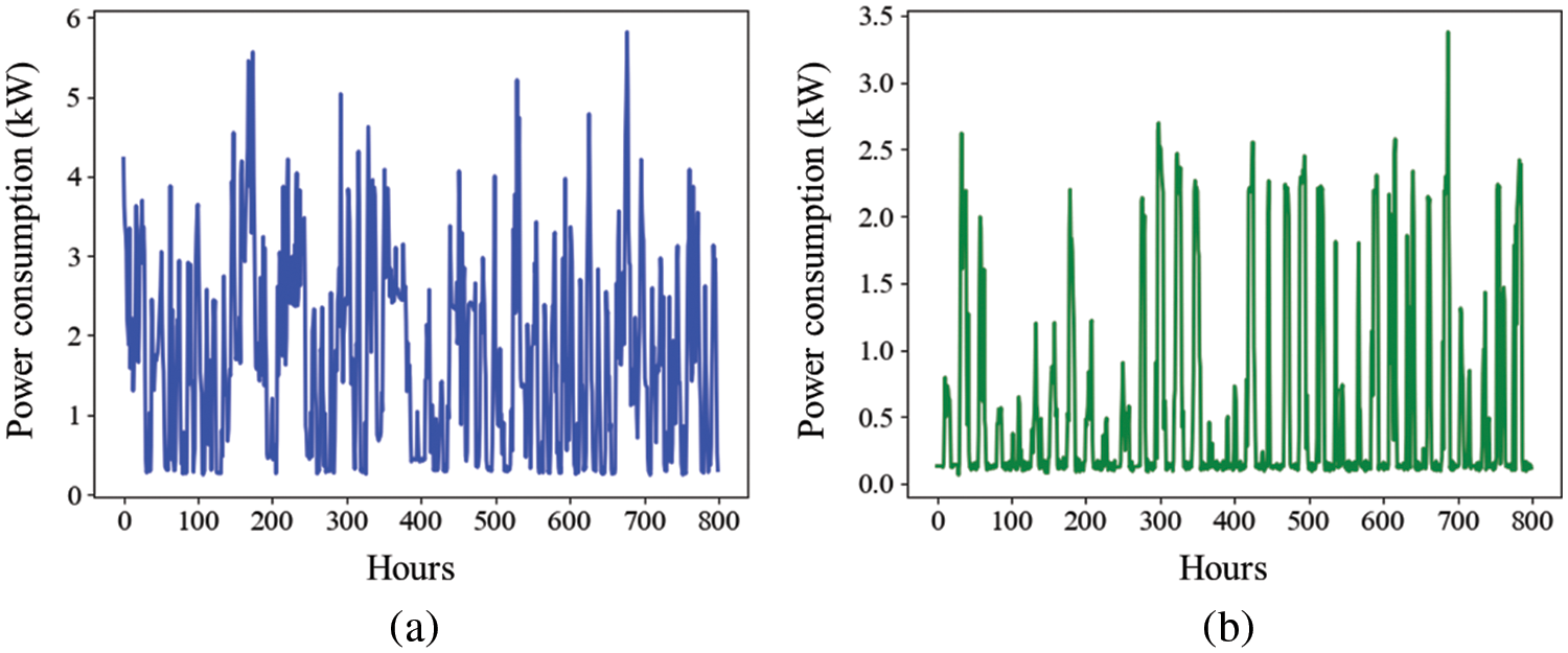
Figure 3: Power consumption datasets samples (a) IHEPC residential building data, (b) AICT commercial building data

4.3 Comparative Analysis with SOTA

This section provides a detailed discussion of the assessment of the proposed model and other recent SOTA PC forecasting networks. The results obtained by the proposed and other recent SOTA are presented in Table 4 where the last row illustrates our model’s results while the remaining rows provide the comparative networks. In this regard, we compare the proposed method with [55] in which the authors used CNN and LSTM-based end-to-end model for PC forecasting in the residential home by obtaining the MSE, MAE, and RMSE values 0.3549, 0.3317, and 0.5957, respectively. Next, CNN and GRU-based network introduced in [63] is also compared where their error values are 0.4700, 0.3300, and 0.2200 for RMSE, MAE, and MSE, respectively. In another study [64], the CNN and LSTM-based AE are combined and a hybrid model is introduced that achieved the error metrics such as MAE, MSE, and RMSE values 0.3100, 0.1900, and 0.4700, respectively. A multilayer GRU network is developed in [65] to predict the short-term PC and achieved the error values 0.1900, 0.1700, and 0.2200 for MAE, MSE, and RMSE, respectively. In the study [66], CNN is combined with bidirectional GRU and made a CNN-BGRU network for load forecasting in residential houses where the model gets the MAE, MSE, and RMSE values 0.2900, 0.1800, and, 0.4200. Another recent study [67] incorporated convolutional LSTM with stacked GRU for PC prediction, and achieved the error values 0.4882, 0.3435, and 0.2384 for RMSE, MAE, and MSE, respectively. Compared to the SOTA approaches, the proposed model obtains remarkable results, which are 0.0147, 0.1212, and 0.0871 for MSE, RMSE, and MAE, respectively.

4.4 Ablation Study for Model Component Selection

In this section, the effectiveness of each component of the proposed model in terms of error metrics is illustrated. Two main modules in our model that include CNN-based AE and online sequential ELM. Three experiments are performed using these models on the IHEPC and AICT datasets separately. In the first experiment using IHEPC data, the online sequential ELM model is trained and evaluated. The obtained error metrics such as MAE, MSE, R2, AR2, and RMSE are 0.0981, 0.0198, 0.3086, 0.2757, and 0.1407, respectively. Similarly, in the second experiment on the IHEPC dataset, CNN is evaluated by obtaining the error values of 0.0179, 0.0931, 0.3219, 0.3197, and 0.1338 for MSE, MAE, R2, AR2, and RMSE, respectively. The result of CNN is improved compared to online sequential ELM. Finally, in the third experiment, CNN-based AE and online sequential ELM are combined in a hybrid network and used for the evaluation of the IHEPC dataset. The results of the proposed model are 0.1212, 0.0871, 0.3487, 0.3341, and 0.0147 for RMSE, MAE, R2, AR2, and MSE, respectively. All these three models’ results are provided in Table 5 where the online sequential ELM results are improved by CNN and the proposed hybrid model achieved the lowest error rate among all the evaluated models. Next, all three models are also evaluated and compared using the AICT commercial building PC dataset. The MSE values are 0.0195, 0.0168, and 0.0121 for online sequential ELM, CNN, and proposed network respectively while RMSE and MAE values for all the models are given in Table 5. Similarly, for visual comparison of all the models’ predictions are plotted in Figs. 4 and 5 for IHEPC and AICT datasets, respectively. These comparisons show that the combination of CNN-based AE and online sequential ELM produces less error on both datasets. Therefore, we choose it as a proposed model and compare it with SOTA in the above subsection.

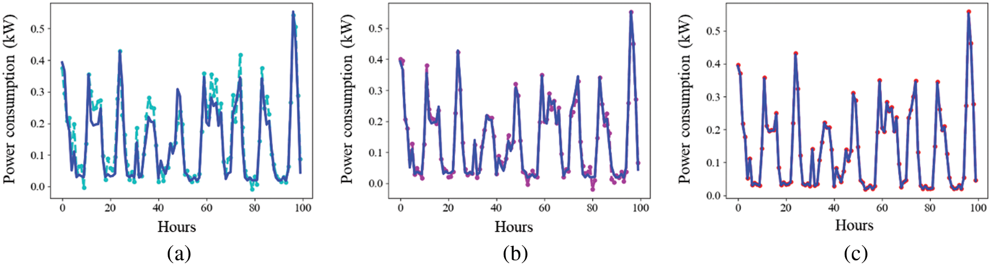
Figure 4: Ablation study models visual prediction results using IHEPC residential data: (a) online sequential ELM, (b) CNN, (c) proposed model

Figure 5: Ablation study models visual prediction results using AICT commercial data: (a) online sequential ELM, (b) CNN, (c) proposed model

5  Conclusion and Future Work

The use of energy is increasing globally due to the advancement in technology, industries, transportation, and population. Commercial and residential buildings are the important consumer of the generated energy. AI-based power management in these buildings can save a large amount of power, and produce productive ways for green energy integration into homes and smart grids. Therefore, in this study, we introduced a novel hybrid model for PC forecasting in residential and commercial buildings. Instead of using complex features engineering approaches, a CNN-based deep AE is used that extracts the efficient compressed spatial features. Next, the representative features are provided to the online sequential ELM that learns the dynamic and temporal relation from the PC data. Finally, the proposed model performance is evaluated on two PC datasets of commercial and residential buildings and also compared with SOTA data-driven networks. Detailed ablation study and comparison prove that our model obtains remarkable performance compared to other approaches. The proposed method produced MAE values of 0.0871 and 0.0887, respectively, for the datasets of residential and commercial structures. The performance of the model reveals that it can be used in smart electric grids, buildings, and energy stations as a trustworthy solution for PC forecasting.

In the future, this work can be extended to the other major sectors of load consumers such as industries and transportation. Future prediction resolution also plays a key role in energy management, therefore we intend to forecast multi-step energy consumption in different resolutions. However, the uncertainties such as noise and anomalies in the industries and transportation PC data exist that need to be handled using an efficient approach. Similarly, motivated by the advancements in IoT technology, the proposed model parameters can be tuned to make them suitable for these networks. In addition, this idea can be integrated with the other domain of energy such as power generation prediction from wind or solar.

Acknowledgement: None.

Funding Statement: This work was supported by the National Research Foundation of Korea (NRF) grant funded by the Korean government (MSIT) (No. 2019M3F2A1073179).

Author Contributions: The authors confirm contribution to the paper as follows: study conception and design: Noman Khan; data collection: Noman Khan, Samee Ullah Khan; analysis and interpretation of results: Noman Khan, Samee Ullah Khan; draft manuscript preparation: Noman Khan; writing review & editing: Noman Khan, Samee Ullah Khan; supervision: Sung Wook Baik. All authors reviewed the results and approved the final version of the manuscript.

Availability of Data and Materials: The authors do not have permission to share data.

Conflicts of Interest: The authors declare that they have no conflicts of interest to report regarding the present study.

References

1. T. Ahmad, R. Madonski, D. Zhang, C. Huang and A. Mujeeb, “Data-driven probabilistic machine learning in sustainable smart energy/smart energy systems: Key developments, challenges, and future research opportunities in the context of smart grid paradigm,” Renewable and Sustainable Energy Reviews, vol. 160, pp. 112128, 2022. [Google Scholar]

2. S. Nathaphan and A. Therdyothin, “Effectiveness evaluation of the energy efficiency and conservation measures for stipulation of Thailand energy management system in factory,” Journal of Cleaner Production, vol. 383, pp. 135442, 2023. [Google Scholar]

3. C. Yu and W. Pan, “Inter-building effect on building energy consumption in high-density city contexts,” Energy and Buildings, vol. 278, pp. 112632, 2023. [Google Scholar]

4. M. Nutakki and S. Mandava, “Review on optimization techniques and role of artificial intelligence in home energy management systems,” Engineering Applications of Artificial Intelligence, vol. 119, pp. 105721, 2023. [Google Scholar]

5. M. Abdel-Basset, H. Hawash, K. Sallam, S. Askar and M. Abouhawwash, “STLF-Net: Two-stream deep network for short-term load forecasting in residential buildings,” Journal of King Saud University-Computer and Information Sciences, vol. 34, no. 7, pp. 4296–4311, 2022. [Google Scholar]

6. H. Shreenidhi and N. S. Ramaiah, “A two-stage deep convolutional model for demand response energy management system in IoT-enabled smart grid,” Sustainable Energy,” Grids and Networks, vol. 30, pp. 100630, 2022. [Google Scholar]

7. M. Lumbreras, R. Garay-Martinez, B. Arregi, K. Martin-Escudero, G. Diarce et al., “Data driven model for heat load prediction in buildings connected to district heating by using smart heat meters,” Energy, vol. 239, pp. 122318, 2022. [Google Scholar]

8. G. F. Fan, L. Z. Zhang, M. Yu, W. C. Hong and S. Q. Dong, “Applications of random forest in multivariable response surface for short-term load forecasting,” International Journal of Electrical Power & Energy Systems, vol. 139, pp. 108073, 2022. [Google Scholar]

9. J. Zhu, H. Dong, W. Zheng, S. Li, Y. Huang et al., “Review and prospect of data-driven techniques for load forecasting in integrated energy systems,” Applied Energy, vol. 321, pp. 119269, 2022. [Google Scholar]

10. R. K. Jagait, M. N. Fekri, K. Grolinger and S. Mir, “Load forecasting under concept drift: Online ensemble learning with recurrent neural network and ARIMA,” IEEE Access, vol. 9, pp. 98992–99008, 2021. [Google Scholar]

11. G. Sideratos, A. Ikonomopoulos and N. D. Hatziargyriou, “A novel fuzzy-based ensemble model for load forecasting using hybrid deep neural networks,” Electric Power Systems Research, vol. 178, pp. 106025, 2020. [Google Scholar]

12. L. Zhang, J. Wen, Y. Li, J. Chen, Y. Ye et al., “A review of machine learning in building load prediction,” Applied Energy, vol. 285, pp. 116452, 2021. [Google Scholar]

13. A. S. Khwaja, A. Anpalagan, M. Naeem and B. Venkatesh, “Joint bagged-boosted artificial neural networks: Using ensemble machine learning to improve short-term electricity load forecasting,” Electric Power Systems Research, vol. 179, pp. 106080, 2020. [Google Scholar]

14. K. Li, J. Zhang, X. Chen and W. Xue, “Building’s hourly electrical load prediction based on data clustering and ensemble learning strategy,” Energy and Buildings, vol. 261, pp. 111943, 2022. [Google Scholar]

15. W. Zhou, X. Min, Y. Zhao, Y. Pang and J. Yi, “A multi-scale spatio-temporal network for violence behavior detection,” IEEE Transactions on Biometrics, Behavior, and Identity Science, 2023. [Google Scholar]

16. Q. Yuan, K. Chen, Y. Yu, N. Q. K. Le and M. C. H. Chua, “Prediction of anticancer peptides based on an ensemble model of deep learning and machine learning using ordinal positional encoding,” Briefings in Bioinformatics, vol. 24, no. 1, bbac630, 2023. [Google Scholar] [PubMed]

17. Y. Lu, M. Khan and M. D. Ansari, “Face recognition algorithm based on stack denoising and self-encoding lbp,” Journal of Intelligent Systems, vol. 31, no. 1, pp. 501–510, 2022. [Google Scholar]

18. S. Yuan, Y. Chen, C. Ye and M. D. Ansari, “Edge detection using nonlinear structure tensor,” Nonlinear Engineering, vol. 11, no. 1, pp. 331–338, 2022. [Google Scholar]

19. N. Taleb, S. Mehmood, M. Zubair, I. Naseer, B. Mago et al., “Ovary cancer diagnosing empowered with machine learning,” 2022 Int. Conf. on Business Analytics for Technology and Security (ICBATS), Dubai, United Arab Emirates, pp. 1–6, 2022. [Google Scholar]

20. M. U. Nasir, S. Khan, S. Mehmood, M. A. Khan, A. U. Rahman et al., “IoMT-Based osteosarcoma cancer detection in histopathology images using transfer learning empowered with blockchain, fog computing, and edge computing,” Sensors, vol. 22, no. 14, pp. 5444, 2022. [Google Scholar] [PubMed]

21. M. U. Nasir, S. Khan, S. Mehmood, M. A. Khan, M. Zubair et al., “Network meddling detection using machine learning empowered with blockchain technology,” Sensors, vol. 22, no. 18, pp. 6755, 2022. [Google Scholar] [PubMed]

22. S. C. Nayak and M. D. Ansari, “COA-HONN: Cooperative optimization algorithm based higher order neural networks for stock forecasting,” Recent Advances in Computer Science and Communications (Formerly: Recent Patents on Computer Science), vol. 14, no. 7, pp. 2376–2392, 2021. [Google Scholar]

23. S. C. Nayak, S. Das and M. D. Ansari, “TLBO-FLN: Teaching-learning based optimization of functional link neural networks for stock closing price prediction,” International Journal of Sensors Wireless Communications and Control, vol. 10, no. 4, pp. 522–532, 2020. [Google Scholar]

24. R. Abiyev and S. Abizada, “Type-2 fuzzy wavelet neural network for estimation energy performance of residential buildings,” Soft Computing, vol. 25, no. 16, pp. 11175–11190, 2021. [Google Scholar]

25. Z. Wang, T. Hong and M. A. Piette, “Building thermal load prediction through shallow machine learning and deep learning,” Applied Energy, vol. 263, pp. 114683, 2020. [Google Scholar]

26. C. Li, “Designing a short-term load forecasting model in the urban smart grid system,” Applied Energy, vol. 266, pp. 114850, 2020. [Google Scholar]

27. B. Dietrich, J. Walther, M. Weigold and E. Abele, “Machine learning based very short term load forecasting of machine tools,” Applied Energy, vol. 276, pp. 115440, 2020. [Google Scholar]

28. C. Liu, B. Sun, C. Zhang and F. Li, “A hybrid prediction model for residential electricity consumption using holt-winters and extreme learning machine,” Applied Energy, vol. 275, pp. 115383, 2020. [Google Scholar]

29. Y. Dai and P. Zhao, “A hybrid load forecasting model based on support vector machine with intelligent methods for feature selection and parameter optimization,” Applied Energy, vol. 279, pp. 115332, 2020. [Google Scholar]

30. R. J. Park, K. B. Song and B. S. Kwon, “Short-term load forecasting algorithm using a similar day selection method based on reinforcement learning,” Energies, vol. 13, no. 10, pp. 2640, 2020. [Google Scholar]

31. K. Nam, S. Hwangbo and C. Yoo, “A deep learning-based forecasting model for renewable energy scenarios to guide sustainable energy policy: A case study of korea,” Renewable and Sustainable Energy Reviews, vol. 122, pp. 109725, 2020. [Google Scholar]

32. X. Liu, Z. Zhang and Z. Song, “A comparative study of the data-driven day-ahead hourly provincial load forecasting methods: From classical data mining to deep learning,” Renewable and Sustainable Energy Reviews, vol. 119, pp. 109632, 2020. [Google Scholar]

33. G. Chitalia, M. Pipattanasomporn, V. Garg and S. Rahman, “Robust short-term electrical load forecasting framework for commercial buildings using deep recurrent neural networks,” Applied Energy, vol. 278, pp. 115410, 2020. [Google Scholar]

34. L. Yin and J. Xie, “Multi-temporal-spatial-scale temporal convolution network for short-term load forecasting of power systems,” Applied Energy, vol. 283, pp. 116328, 2021. [Google Scholar]

35. M. Imani and H. Ghassemian, “Residential load forecasting using wavelet and collaborative representation transforms,” Applied Energy, vol. 253, pp. 113505, 2019. [Google Scholar]

36. Q. Xu, X. Yang and X. Huang, “Ensemble residual networks for short-term load forecasting,” IEEE Access, vol. 8, pp. 64750–64759, 2020. [Google Scholar]

37. Y. He, P. Wu, Y. Li, Y. Wang, F. Tao et al., “A generic energy prediction model of machine tools using deep learning algorithms,” Applied Energy, vol. 275, pp. 115402, 2020. [Google Scholar]

38. J. Li, D. Deng, J. Zhao, D. Cai, W. Hu et al., “A novel hybrid short-term load forecasting method of smart grid using MLR and LSTM neural network,” IEEE Transactions on Industrial Informatics, vol. 17, no. 4, pp. 2443–2452, 2020. [Google Scholar]

39. A. Heydari, M. M. Nezhad, E. Pirshayan, D. A. Garcia, F. Keynia et al., “Short-term electricity price and load forecasting in isolated power grids based on composite neural network and gravitational search optimization algorithm,” Applied Energy, vol. 277, pp. 115503, 2020. [Google Scholar]

40. Y. Wang, J. Chen, X. Chen, X. Zeng, Y. Kong et al., “Short-term load forecasting for industrial customers based on TCN-LightGBM,” IEEE Transactions on Power Systems, vol. 36, no. 3, pp. 1984–1997, 2020. [Google Scholar]

41. F. He, J. Zhou, L. Mo, K. Feng, G. Liu et al., “Day-ahead short-term load probability density forecasting method with a decomposition-based quantile regression forest,” Applied Energy, vol. 262, pp. 114396, 2020. [Google Scholar]

42. G. Hafeez, K. S. Alimgeer and I. Khan, “Electric load forecasting based on deep learning and optimized by heuristic algorithm in smart grid,” Applied Energy, vol. 269, pp. 114915, 2020. [Google Scholar]

43. X. Kong, C. Li, C. Wang, Y. Zhang and J. Zhang, “Short-term electrical load forecasting based on error correction using dynamic mode decomposition,” Applied Energy, vol. 261, pp. 114368, 2020. [Google Scholar]

44. N. Somu, G. R. MR and K. Ramamritham, “A hybrid model for building energy consumption forecasting using long short term memory networks,” Applied Energy, vol. 261, pp. 114131, 2020. [Google Scholar]

45. L. Cascone, S. Sadiq, S. Ullah, S. Mirjalili, H. U. R. Siddiqui et al., “Predicting household electric power consumption using multi-step time series with convolutional LSTM,” Big Data Research, vol. 31, pp. 100360, 2023. [Google Scholar]

46. J. Munkhammar, D. van der Meer and J. Widén, “Very short term load forecasting of residential electricity consumption using the Markov-chain mixture distribution (MCM) model,” Applied Energy, vol. 282, pp. 116180, 2021. [Google Scholar]

47. A. Gellert, A. Florea, U. Fiore, F. Palmieri and P. Zanetti, “A study on forecasting electricity production and consumption in smart cities and factories,” International Journal of Information Management, vol. 49, pp. 546–556, 2019. [Google Scholar]

48. L. Xu, J. Pan, R. Wang, Y. Tao, Y. Guo et al., “Prediction of the total day-round thermal load for residential buildings at various scales based on weather forecast data,” Applied Energy, vol. 280, pp. 116002, 2020. [Google Scholar]

49. N. Fumo and M. R. Biswas, “Regression analysis for prediction of residential energy consumption,” Renewable and Sustainable Energy Reviews, vol. 47, pp. 332–343, 2015. [Google Scholar]

50. A. Gellert, U. Fiore, A. Florea, R. Chis and F. Palmieri, “Forecasting electricity consumption and production in smart homes through statistical methods,” Sustainable Cities and Society, vol. 76, pp. 103426, 2022. [Google Scholar]

51. H. Takeda, Y. Tamura and S. Sato, “Using the ensemble kalman filter for electricity load forecasting and analysis,” Energy, vol. 104, pp. 184–198, 2016. [Google Scholar]

52. Y. Zhou, C. Lork, W. T. Li, C. Yuen and Y. M. Keow, “Benchmarking air-conditioning energy performance of residential rooms based on regression and clustering techniques,” Applied Energy, vol. 253, pp. 113548, 2019. [Google Scholar]

53. Y. Chen, P. Xu, Y. Chu, W. Li, Y. Wu et al., “Short-term electrical load forecasting using the support vector regression (SVR) model to calculate the demand response baseline for office buildings,” Applied Energy, vol. 195, pp. 659–670, 2017. [Google Scholar]

54. A. Bogomolov, B. Lepri, R. Larcher, F. Antonelli, F. Pianesi et al., “Energy consumption prediction using people dynamics derived from cellular network data,” EPJ Data Science, vol. 5, pp. 1–15, 2016. [Google Scholar]

55. T. Y. Kim and S. B. Cho, “Predicting residential energy consumption using CNN-LSTM neural networks,” Energy, vol. 182, pp. 72–81, 2019. [Google Scholar]

56. Z. Xiao, W. Gang, J. Yuan, Z. Chen, J. Li et al., “Impacts of data preprocessing and selection on energy consumption prediction model of HVAC systems based on deep learning,” Energy and Buildings, vol. 258, pp. 111832, 2022. [Google Scholar]

57. D. Yang, J. E. Guo, S. Sun, J. Han and S. Wang, “An interval decomposition-ensemble approach with data-characteristic-driven reconstruction for short-term load forecasting,” Applied Energy, vol. 306, pp. 117992, 2022. [Google Scholar]

58. S. Cantero-Chinchilla, C. A. Simpson, A. Ballisat, A. J. Croxford and P. D. Wilcox, “Convolutional neural networks for ultrasound corrosion profile time series regression,” NDT & E International, vol. 133, pp. 102756, 2023. [Google Scholar]

59. Y. Wei, J. Jang-Jaccard, W. Xu, F. Sabrina, S. Camtepe et al., “LSTM-autoencoder based anomaly detection for indoor air quality time series data,” IEEE Sensors Journal, vol. 23, no. 4, pp. 3787–3800, 2023. [Google Scholar]

60. P. Li, B. Anduv, X. Zhu, X. Jin and Z. Du, “Diagnosis for the refrigerant undercharge fault of chiller using deep belief network enhanced extreme learning machine,” Sustainable Energy Technologies and Assessments, vol. 55, pp. 102977, 2023. [Google Scholar]

61. M. Jamei, I. Ahmadianfar, M. Karbasi, A. Malik, O. Kisi et al., “Development of wavelet-based kalman online sequential extreme learning machine optimized with boruta-random forest for drought index forecasting,” Engineering Applications of Artificial Intelligence, vol. 117, pp. 105545, 2023. [Google Scholar]

62. G. Hebrail and A. Berard, “Individual household electric power consumption,” in UCI machine learning repository, Irvine, CA: University of California, School of Information and Computer, 2012. [Google Scholar]

63. M. Sajjad, Z. A. Khan, A. Ullah, T. Hussain, W. Ullah et al., “A novel CNN-GRU-based hybrid approach for short-term residential load forecasting,” IEEE Access, vol. 8, pp. 143759–143768, 2020. [Google Scholar]

64. Z. A. Khan, T. Hussain, A. Ullah, S. Rho, M. Lee et al., “Towards efficient electricity forecasting in residential and commercial buildings: A novel hybrid CNN with a LSTM-AE based framework,” Sensors, vol. 20, no. 5, pp. 1399, 2020. [Google Scholar] [PubMed]

65. T. Han, K. Muhammad, T. Hussain, J. Lloret and S. W. Baik, “An efficient deep learning framework for intelligent energy management in IoT networks,” IEEE Internet of Things Journal, vol. 8, no. 5, pp. 3170–3179, 2020. [Google Scholar]

66. Z. A. Khan, A. Ullah, W. Ullah, S. Rho, M. Lee et al., “Electrical energy prediction in residential buildings for short-term horizons using hybrid deep learning strategy,” Applied Sciences, vol. 10, no. 23, pp. 8634, 2020. [Google Scholar]

67. F. U. M. Ullah, A. Ullah, N. Khan, M. Y. Lee, S. Rho et al., “Deep learning-assisted short-term power load forecasting using deep convolutional LSTM and stacked GRU,” Complexity, vol. 2022, pp. 2993184, 2022. [Google Scholar]