
 Submit a Paper
 Propose a Special lssue
 Open Access
ARTICLE

Study on Flow Field Simulation at Transmission Towers in Loess Hilly Regions Based on Circular Boundary Constraints
1 Electric Power Research Institute, State Grid Shanxi Electric Power Company, Taiyuan, 030001, China
2 School of Electrical Engineering, Xi’an Jiaotong University, Xi’an, 710049, China
3 Xi’an North Power Supply Company, State Grid Shaanxi Electric Power Company, Xi’an, 710018, China
* Corresponding Author: Bo He. Email:
(This article belongs to the Special Issue: Wind Energy Development and Utilization)
Energy Engineering 2023, 120(10), 2417-2431. https://doi.org/10.32604/ee.2023.029596
Received 27 February 2023; Accepted 05 May 2023; Issue published 28 September 2023
 View Full Text
 Download PDF
Abstract
When using high-voltage transmission lines for energy transmission in loess hilly regions, local extreme wind fields such as turbulence and high-speed cyclones occur from time to time, which can cause many kinds of mechanical and electrical failures, seriously affecting the reliable and stable energy transmission of the power grid. The existing research focuses on the wind field simulation of ideal micro-terrain and actual terrain with mostly single micro-terrain characteristics. Model boundary constraints and the influence of constrained boundaries are the main problems that need to be solved to accurately model and simulate complex flow fields. In this paper, a flow field simulation method based on circular boundary constraints is carried out. During the study, the influence of the model boundary and the selection conditions of the modeling range are systematically analyzed. It is more suitable to make sure that the air domain is 4 times higher than the height of the hill undulations, in addition to ensuring that there should be a minimum of 400 m between the study region and the boundary. Then, an actual terrain model of a power grid line in Shanxi is established, through the method proposed in this paper, the wind speed at the location of the transmission tower line under different wind directions is analyzed, and it is found thatwhen the incidence direction is 45 degrees north by east the wind speed is the highest. The findings demonstrate that the circular boundary model has the advantage of more easily adjusting the wind incidence direction, in addition to theoretically reducing the errors caused by traditional models in boundary processing. It can accurately obtain the distribution characteristics of the flow field affected by the terrain, and quickly screen out the extreme working conditions that are most harmful to the transmission lines in the actual transmission line for energy transmission in complex loess hilly regions.Keywords
Nomenclature
| δ | Wind speed change caused by boundary change/m·s−1 |
| Average wind speed/m·s−1 | |
| Average wind speed at standard height/m·s−1 | |
| Height/m | |
| Standard height/m | |
| Surface roughness coefficient | |
| k | Turbulent kinetic energy/m2·s−2 |
| I | Intensity of turbulence |
| Lu | Integral scale of turbulence/m |
| z0 | Roughness length/m |
| k0 | Roughness height/m |
| ε | Turbulence dissipation rate/m2·s−3 |
The surface of the loess hilly regions is full of gullies and complex in structure. The macro wind speed, wind direction, and other meteorological data are constantly evolving under the influence of the gullies on the surface of the loess hilly regions, which makes it easy to produce various types of turbulence and high-speed cyclones [1–3]. In most cases, the wind speed, wind direction, and pulsation characteristics are significantly different from the macro meteorological data in strong convective micrometeorology. For the operation and maintenance of high-voltage transmission lines in loess hilly regions, the meteorological data of such terrain is often a blind area that cannot be covered by comprehensive meteorological data monitoring. Extreme changes in wind fields caused by the local microtopography can seriously compromise the stability and safety of various energy generation, transmission, and usage operations [4–6].
In recent years, various kinds of wind-induced disasters have occurred frequently on power transmission lines in the micro-topographic meteorological area. On July 31, 2021, the western regions of Handan experienced a short-time severe convective weather, which caused damages to 21 lines in total. On November 21, 2021, severe convective weather hit parts of Ningwu County, Shanxi Province, causing damage to several high-voltage power transmission lines. The local strong convective climate affected by microtopography has seriously affected the reliability of high-voltage transmission lines.
At present, three main research methods of flow fields have been developed [7–11]. On-site measurement of the actual micro-terrain area is the most direct method. However, this method has a high cost. In addition, due to the influence of actual terrain, wind speed and other factors, the grid of wind measurement points is sparse. This phenomenon means that it is difficult to generalize rules for terrain features, and wind maps can be rough. The wind tunnel test method based on the microtopographic scaling model also has the characteristics of high difficulty in model making, long test cycles, and difficulties to eliminate the influence of flow field boundary.
In contrast, simulation analysis has many advantages such as flexibility, efficiency, and low cost, and its technology has developed rapidly [12]. Jackson et al. [13,14] and Hunt et al. [15] proposed and perfected the functional formula for calculating the rate of change of wind speed at the top of a two-dimensional mountain in the 1970s. Then the research on wind field simulation using numerical simulation methods continued to develop. Zhou et al. [16] studied the application of the Realizable k-ε model in the calculation of the partial working condition of hydro turbines, and believed that the model satisfies the Reynolds stress constraint condition and can more accurately simulate the diffusion speed of the plane and circular jets. Li [17] used the Realizable k-ε model to simulate the wind field numerically and held the view that the model was closer to the actual situation in the wind field simulation. Gao et al. [18] adopted a closed treatment for the turbulent Navier-Stokes equation in the steady-state situation and obtained the corresponding numerical solution by discretizing the microtopographic wind field. Sun et al. [19] conducted simulations of turbines in wind fields using the realizable k-ε model to investigate the impact of walls on downstream wind speed changes.
As far as the current simulation analysis of wind response of high-voltage transmission lines is concerned, researchers have made significant advancements in the development of finite element models, the analysis of wind load characteristics and dynamic behavior, and the probability distribution of tower line systems [20–22]. Some previous research focused mainly on the effects of typical ideal terrain on wind fields [23,24]. Such research idealizes the structure of mountains, abstracts the various shapes of mountain bodies in nature into ideal geometry models. However, in actual circumstances, the terrain of the loess hilly regions is so complex that it cannot simply be analyzed and interpreted using an ideal terrain or a local terrain, and many actual geological problems cannot be solved. Other previous research focuses on the wind field simulation of actual terrain with only single micro-terrain characteristics, such as a mountain or a hilly terrain, and they generally use a rectangular boundary model similar to a wind tunnel [25–28]. Such a method can be used in some simple terrain areas. The area in which the real transmission tower line is located may be affected by different complex terrains and the wind speed results are completely different from the results of the simple terrain analysis. The parts between the real terrain and the rectangular air domains generally adopt a functionally smooth approach, thereby introducing unnecessary errors. Rectangular boundary constraints also have certain limitations when studying different wind direction angles. In the case where the wind speed is incident perpendicular to the rectangular boundary, the constraints of the side boundary will affect the wind field simulation results. It is common practice to apply constraints simultaneously on adjacent rectangular boundaries when changing the direction of the wind speed. This method of imposing constraints is not only complex but also introduces relatively large errors.
To solve the problem mentioned above, this paper proposes a large-field wind field simulation method with circular boundary constraints. It provides an easier solution to study the influence of different wind incidence angles under complex terrain.
In this paper, the actual terrain model of the 220 kV transmission line in Yuncheng, Shanxi Province is selected as the research object. Moreover, eight wind incidence angles of 0°, 45°, 90°, 135°, 180°, 225°, 270°, and 315° are set to study the distortion effect of the terrain distribution under different wind incidence angles.
2 Establishment of Wind Field Simulation Model
2.1 Actual Terrain of the Study
In order to better simulate the wind field of the transmission tower line in the actual complex terrain, this paper selects a typical loess hilly region near 35°29′N and 111°10′E in Yuncheng, Shanxi Province for study, as shown in Fig. 1.

Figure 1: Actual topographic map of Yuncheng, Shanxi Province
As can be seen from Fig. 1, there are two crisscrossing sections in this area, including a hill extending from southwest to northeast on the west side and a set of hills extending from northwest to southeast on the east side. Transmission tower No. 55 of the Xinren line (that is, the location marked in the map) is in a ravine terrain between these hills. The geographical structure is complex, which is a typical loess hilly ravine. In such a topographic environment, local strong convective micro-meteorological regions are prone to occur, resulting in wind speed and wind direction that are significantly different from the macro-meteorological data in Yuncheng. Therefore, this location selected for research can reflect the influence of local microtopography on the wind field.
2.2 Modeling Ranges for Circular Terrain Models
2.2.1 Heights of Circular Terrain Modeling
To reduce the influence of boundaries during wind simulation, a series of circular terrain models with the same radius and different heights are established. The heights of the air domains z were taken as 600, 800, and 1000 m, respectively. The hill undulations in the selected area vary by about 200 m, that is, the heights of the established air domains are 3, 4 and 5 times the terrain height, respectively.
Use Ansys Fluent to conduct wind field simulation on the established model, keep the rest of the simulation settings consistent, set the inlet wind speed to 25 m/s, and the direction is directed along the x-axis to the negative direction of the x-axis. For different heights, wind field calculations are performed separately, and then the same position is selected in the center of the model. From the datawithin 450 m from the ground, the relationship between wind speed and height from the ground is obtained, as shown in Fig. 2.

Figure 2: Wind speed at different modeling heights
From Fig. 2, it can be seen that the increase in model height from 600 to 800 m has a relatively large impact on wind simulation, while the impact on wind simulation is negligible when the model height increases from 800 to 1000 m. To determine this regularity, the air domain height of the model is set to 2000 m (that is, 10 times the height of hill undulation) for wind field calculation, and the results are added to Fig. 2. As can be seen from Fig. 2, from 1000 to 2000 m, the wind speed change is not significant even if the height increases by 1000 m.
In order to quantitatively describe the change of wind speed with height in Fig. 2, define the amount of wind speed change caused by the height change in the air domain as δ. It is used to measure the relationship between the wind speed difference under different conditions and the model height multiple difference. The mathematical expression is as follows:
It is known by calculation that the average wind speed change of each point reaches 0.93 m/s when the model height increases from 600 to 800 m, and the average change decreases to 0.18 m/s when the model height increases from 800 to 1000 m. The influence of increasing the model height on the wind field change in the model decreases. During the increase in model height from 1000 to 2000 m, the average change decreased to 0.08 m/s. It can be concluded that the influence of increasing the height of the model air domain on the wind field will decrease with the increase of the height of the model air domain.
Therefore, in order to reduce the calculation amount while ensuring the calculation accuracy, it is more appropriate to select the height of the model air domain as 4 times the hill undulation height.
2.2.2 Radius for Modeling Circular Terrain
The limitation of boundary conditions in wind field simulation will cause errors between the simulation results near the boundary and the actual situation. The closer the position to the internal area of the model, the closer the calculation results are to the real situation. In order to explore the specific scope affected by the boundary of the circular area model, a series of circular 3D models with the same height and different radii of the model air domain were established, with radii of 400, 500, 600, 700 and 800 m, respectively.
Use Ansys Fluent to conduct wind field simulation on the established model, keep the rest of the simulation settings consistent, set the inlet wind speed to 25 m/s, and the direction is directed along the x-axis to the negative direction of the x-axis. For different radii, wind field calculations are performed separately, and then the same position is selected in the center of the model. From the data within450 m from the ground, the relationship between wind speed and height from the ground is obtained, as shown in Fig. 3.
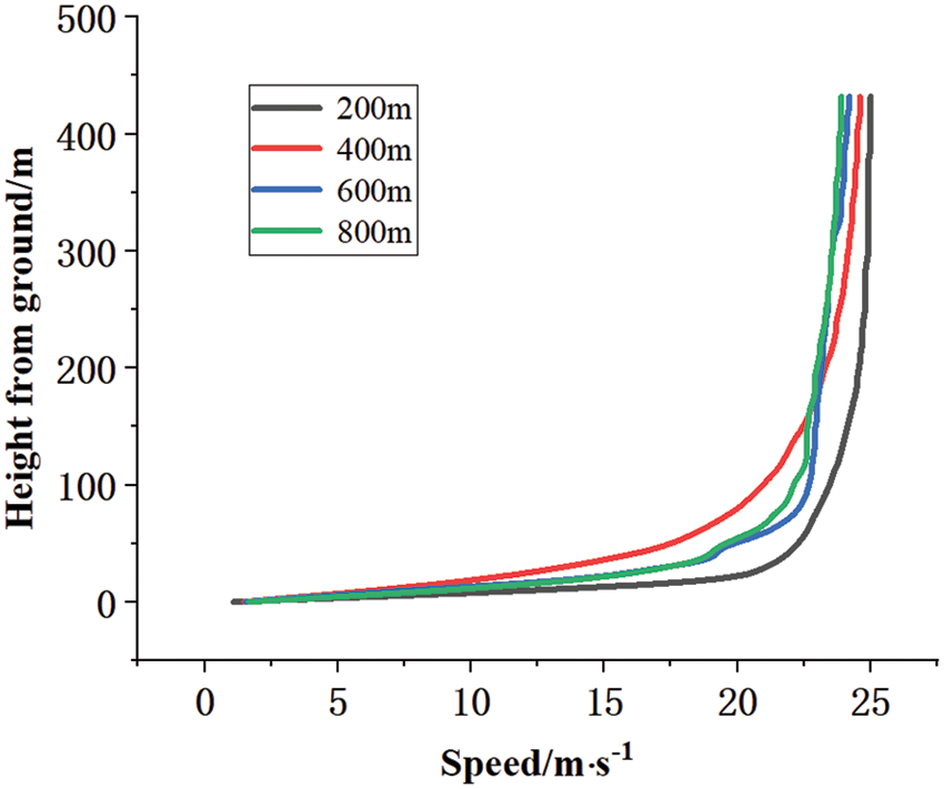
Figure 3: Wind speed under different modeling radii
From Fig. 3, it can be seen that the increase in the radius of the model from 200 to 600 m has a relatively large impact on the wind field simulation. However, the impact on the wind field simulation is relatively small when the model height is increased from 600 to 800 m. This change can be quantitatively expressed by the wind speed change value δ defined above. After calculation, the average wind speed change of each point is greater than 3 m/s when the model radius increases from 200 to 400 m. When the model height increases from 400 to 600 m, the average change decreases to less than 1 m/s. And the average change decreases to 0.4 m/s when the model radius increases from 600 to 800 m. It shows that increasing the model radius will still have an impact on the wind field simulation, but the impact continues to weaken with the increase of the model radius.
Therefore, the error between the result and the actual situation when the radius is less than 400 m from the boundary can be large, while it is very small and can be ignored when the radius is more than 600 m from the boundary.
2.3 Establishment of a Three-Dimensional Terrain Model with a Circular Boundary
According to the research in Part 1.2, the accuracy and calculation of the simulation should be considered. As the topographic elevation map shown in Fig. 4, a circular area with a radius of 1000 m is selected, and the height of the top of the model from the terrain surface is set to 800 m. The direction of wind incidence is also marked in Fig. 4, and the direction in the negative direction of the x-axis is 0°. Rotate a certain angle counterclockwise to obtain other directions of wind incidence, such as the 45° direction marked in Fig. 4.

Figure 4: Round boundary topographic elevation map
Converting elevation data into a 3D terrain model is mainly done through Delaunay triangulation. Currently, the Incremental inserting algorithm is the most commonly used algorithm for Delaunay triangulation, which has simple principle, less memory resources, moderate time complexity, and good segmentation effect [29,30]. Delaunay triangulation is first realized in plane coordinates, and then the height data corresponding to these split nodes is given to form a three-dimensional triangular split terrain mesh surface. The main finite element modeling steps for circular 3D terrain with Ansys are shown in Fig. 5.

Figure 5: Steps of 3D terrain modeling for circular boundary
3 Flow Field Simulation in Loess Hilly Areas
3.1 Test for Grid Independence
The irrelevance of meshing needs to be checked before wind simulation. Use Ansys Fluent to conduct wind field simulation on the established model, keep the direction of incidence and inlet wind speed unchanged, gradually refine the mesh, and calculate the model. To judge the irrelevance of the calculation results to the mesh, compare the calculation results under different mesh accuracy conditions. After calculation, the influence on the results after the mesh accuracy reaches 20 m is negligible. It can be considered that the mesh-independent solution has been obtained.
3.2 Boundary Condition Settings
The circular boundary model can divide the side boundary surface into two semicircles as the inlet surface and outlet surface. It is not only simple to set up but also less affected by boundary constraints inside the model than the rectangular boundary model with four side faces. Before the wind field simulation, the boundary conditions of the circular air domain need to be set, mainly including the inlet surface, the outlet surface, the top surface, and the bottom surface.
3.2.1 Radius for Modeling Circular Terrain
This article sets the inlet face of the air domain as the speed inlet in Ansys Fluent to conduct wind field simulation. The direction of wind speed at the speed inlet can be changed by rotating the inlet surface. Moreover, the average wind speed at the inlet, turbulent kinetic energy and its dissipation rate can be set by writing user-defined functions.
The average wind speed at the speed inlet is described using the exponential law which was first proposed by G. Hellman in 1916. A.G. Davenport of Canada [31] obtained the expression of the exponential law wind profile after a large number of field observations and statistical analysis. In general, the average wind speed
where
The turbulent energy of the inlet face and the turbulent dissipation rate are functions of height, like the wind speed of the inlet face [34]. The turbulent kinetic energy for the inlet face is:
where k(y) is the turbulent kinetic energy at height y, V(y) is the average wind speed at height y, I(y) is the intensity of turbulence at height y, which can be calculated as:
where
where
3.2.2 Outlet Surface and Top Surface
The details of flow speed and pressure are not known prior to solving the flow problem in circular boundary constraint. To avoid the restriction of the outlet surface affecting the flow of wind, this paper sets the outlet surface as outflow boundary conditions, so that the simulation results of the wind speed field can be more accurate. Also, the model has chosen a suitable height, so the wind direction at the top of the model hardly changes, but flows smoothly. To avoid additional boundary conditions that produce different calculations than the wind field of the actual terrain, this paper directly sets the top surface of the air domain as symmetry boundary conditions.
The actual three-dimensional topography of the loess hilly regions constitutes the bottom surface of the air domain. To facilitate further description of the roughness in the simulation process, this paper sets the bottom surface as wall boundary conditions in Ansys Fluent to bound fluid and solid regions, at the same time, uses the standard wall function without specifying shear to describe it.
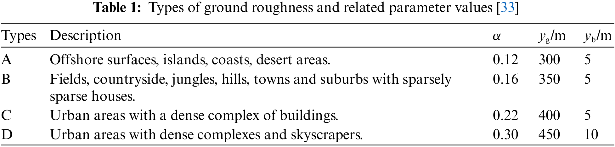
The surface roughness coefficient (α) and the roughness length (
The roughness height of the ground in the Fluent simulation environment setting also describes the roughness of the ground. The conversion relationship between the rough ground height
That is, at the roughness of type B ground studied in this paper, the roughness height
3.3 Flow Fields Simulation with Different Wind Angles
In the model of circular boundaries, the wind incidence angle can be changed by simply changing the position of the division between the inlet and outlet surfaces. It is no longer necessary to calculate the magnitude of components in different directions as in the model of rectangular boundaries, which jointly changes the settings of two adjacent boundary surfaces to achieve a change in wind direction. To study the difference under different wind incidence angle conditions, the direction is changed sequentially by changing the position of the inlet surface and the outlet surface. The direction of wind incidence should be perpendicular to the dividing line between the inlet surface and the outlet surface. Starting from 0° in the wind direction angle, rotate counterclockwise to obtain the wind incidence angle of 45°, 90°, 135°, 180°, 225°, 270°, and 315°.
The gravitational acceleration is set to 9.8 m/s2 before the simulation. The 3D Realizable k-ε model is used for steady-state calculations, and the fluid material is set to “air” to more clearly demonstrate the mathematical and physical characteristics of the flow field. After setting up, initialize and then start the iterative simulation. When the residual reaches the order of
4.1 The Effect of Different Wind Paths on Wind Speed
Use the CFD-Post module to export the wind speed data of the plane passing through the center of the circle at different wind incidence angles. Then obtain the cloud map and vector illustration of wind speed directions, taking 90° and 270° as examples, as shown in Fig. 6.

Figure 6: Wind velocity in different angles of incidence
Fig. 6 shows that the plane passing through the center of the circular terrain model is the same at 90° and 270°. However, the wind speed cloud map and the wind vector illustration of this plane are different because of different wind paths.
From the wind speed cloud map, the wind speed is the same away from the ground in both directions. The maximum wind speeds of both directions, which are 52.12 and 52.58 m/s, appear in the top regions of the model, and it can be assumed that there is no difference. This part of the wind speed is determined by the gradient wind speed at the entrance and is basically not affected by the terrain. The wind speed in some parts near the loess hills has a relatively large difference, which is determined by the different terrain undulations.
Combined with the wind direction vector map, at 90°, the wind path directions are from right to left. The wind rises on the right side of the hill (windward slope) and drops on the left side of the hill (leeward slope). There are obvious vertical wind velocity components on both sides of the hill, which will affect the transmission tower line. The vertical component of the windward slope is upward, and the vertical component of the leeward slope is downward. The closer to the top of the hill, the denser the wind vector and the greater the wind speed. At 270°, the wind path directions are from left to right. Therefore, the path that is a windward slope at 90° is now a leeward slope. The wind rises on the left side of the hill and drops on the right side of the hill. The higher the windward slope rises, the stronger the wind speed accelerates. The greater the leeward slope drops, the larger the low wind speed area behind the hill. The path of wind rises larger than it drops at 90°, while it rises smaller than it drops at 270°. So smaller speeds and lower regions can be found behind the leeward slope at 90° and higher speeds can be found at the top of the mountain at 270°. These laws are consistent with the existing basic topographic structure on the wind field.
4.2 Influence of Different Wind Incidence Directions on Wind Field at an Actual Tower
For the actual terrain, the wind incident from different directions will lead to different travel paths. Through different terrain, different wind fields will be generated at the tower location. The wind field simulation results of the whole regions under different wind directions can be obtained through the wind field simulation calculation. The location of transmission tower No. 55 of Xinren Line is selected for research where the wind field will have some impact on the transmission tower line. The local elevation contour map of the terrain near the transmission tower is shown in Fig. 7.

Figure 7: Local enlarged view of the study terrain
The triangular position in Fig. 7 shows the location of the transmission tower No. 55. It can be seen that the location is in a complex loess hilly terrain combined with the overall topographic analysis, the valley above this terrain is a narrow valley terrain along the left and right direction, similar to the typical canyon wind channel terrain for the lateral incidence direction, and the hills terrain below.
Considering the height of the transmission tower, the wind speed variation within 50 m above the ground at different wind angles is obtained, as shown in Fig. 8. It can be seen that since the location is located in a valley, the wind speed near the ground is very low, close to 0. It is irrelevant with different incidence directions. However, with the increase in height, the wind speed of different incidence directions has increased, and the slope is different. Until the height of 50 m from the ground, the wind speed at different angles has been significantly different. It can be seen that different wind incidence directions have different effects on the wind field distribution at tower No. 55. Such results are consistent with wind field simulations in traditional rectangular models and aerodynamic theoretical analysis.

Figure 8: Speed at different incidence angles
This situation occurs mainly because the terrain on the wind’s path changes when changing the direction of the wind.
Unlike other situations, the terrain through which the path of wind passes is considerably raised at 135°. So the vertical wind at the lower position converges with the lateral wind vector here, resulting in a large synthetic wind speed. Therefore, the wind speed, in this case, has increased significantly much more than in other cases.
At 90°, the upright cliff in front of the wind has a blocking effect on the incoming wind, and the wind will collide with the hill. This collision will cause the wind to lose some of its kinetic energy, so the wind speed is minimal in this situation.
For wind paths in other directions, the position of the transmission tower is in the height drop phase. This location is exactly in the low-speed area of the leeward slope, which is affected by the hill, and the wind speed is small. When the incident direction is 180°, it can be seen from the local magnification that the hill body on the side of the path will converge at the transmission tower, resulting in a large wind speed, which is called “the effect of narrow” [36,37]. “The effect of narrow” has a weaker impact on the wind speed than the elevation of the terrain.
It becomes clear after analysis that there are specific angles for an actual terrain. Those angles result in much higher wind speeds than other angles and more hazardous damage to transmission tower lines. This angle that may cause greater damage to transmission tower lines is called the most dangerous wind angle. For Tower 55 studied in this paper, when the wind direction is 45° north by east, which is called the most hazardous wind incidence angle, the wind speed at the tower will be at its highest. So during the operation and maintenance of the line, if there is strong wind in this direction, special attention should be paid in advance. However, for some angles such as the wind coming from the due north direction, there is no need to be too nervous.
The wind speed is affected by various factors such as side hills and ground uplift in complex loess hilly terrain. So, it is difficult to obtain accurate results simply through theoretical analysis. Therefore, it is crucial to establish a realistic and complex terrain model, flexibly change the direction of wind speed incidence, and study the most dangerous wind direction through the circular boundary flow field simulation proposed in this paper. In this way, targeted line operation and maintenance can be carried out in the future to reduce the occurrence of wind induced tower collapses and avoid accident losses.
This paper suggests a method for simulating complex wind fields by generating large circular fields through terrain modeling in combination with three-dimensional terrain modeling. The loess hilly region where the Xinren line runs is chosen as an engineering example to demonstrate that such a method is plausible. This paper leads to the following conclusions:
(1) The specific size of the model will have a great influence on the wind field calculation results in the simulation of circular boundary terrain. It is reasonable to select 4 times the undulating height of the terrain and 1000 m radius for the circular boundary wind field simulation modeling. The method of selecting the modeling scope is also applicable when other model scope selections are used.
(2) By establishing a large-field 3D terrain model of circular boundary for wind field simulation, the model can reduce the influence of rectangular model boundary constraints and be closer to the actual situation. It can also facilitate the adjustment of wind incidence direction. This method is more suitable for simulating complex hilly terrain related to the direction of wind incidence, and the model is proved to be correct after specific case studies.
(3) The wind speed at a given place will vary depending on the direction of the wind and the path it passes through. When the wind direction is 45° north by east, which is called the most hazardous wind incidence angle, the wind speed at the tower will be at its highest for the tower No. 55 examined in this paper. This discovery can prevent specific wind directions in advance during line operation and maintenance, reducing the huge economic losses caused by wind disasters.
Acknowledgement: The authors would like to thank the editor and anonymous reviewers for their valuable comments.
Funding Statement: This work was supported by a State Grid Shanxi Company’s Science and Technology Project—Research on Grid Wind Farm Condition Monitoring of Transmission Lines in Loess Hilly Regions (520530220005).
Author Contributions: The authors confirm contribution to the paper as follows: study conception and design: Yongxin Liu, Bo He; data collection: Gang Yang, Fuwei He; analysis and interpretation of results: Huaiwei Cao, Puyu Zhao, Hua Yu; draft manuscript preparation: Yongxin Liu, Huaiwei Cao. All authors reviewed the results and approved the final version of the manuscript.
Availability of Data and Materials: The terrain data that support the findings of this study are openly available in Geospatial Data Cloud at https://www.gscloud.cn/.
Conflicts of Interest: The authors declare that they have no conflicts of interest to report regarding the present study.
References
1. Hao, S. (2020). Study on spatial pattern of soil and water conservation function in loess hilly region (Master Thesis). Ningxia University, China. [Google Scholar]
2. Lin, S., Xie, J., Deng, J., Qi, M., Chen, N. (2022). Landform classification based on landform geospatial structure—A case study on Loess Plateau of China. International Journal of Digital, 15(1), 1125–1148. [Google Scholar]
3. Zhao, Y., Wang, X. (2021). Research on wind distribution of Shanxi power grid. Shanxi Electric Power, 1, 17–20. [Google Scholar]
4. Xu, Z., Zhang, Z., Dong, S. (2021). Study of countermeasures against wind damage on transmission lines in northwest mountainous areas of Ningxia. Ningxia Electric Power, 222(6), 25–30. [Google Scholar]
5. Chen, T., Liang, Z., Zhang, L., Han, P. (2023). Analysis of anti-overturning stability and reinforcement measures of movable retractable fence of substation under wind load. Power & Energy, 44(1), 15–19. [Google Scholar]
6. Han, X., Gao, Z. (2020). Calculation and analysis of the influence of mountains on wind farms. Power System and Clean Energy, 36(8), 112–115. [Google Scholar]
7. Takahashi, T., Ohtsu, T., Yassin, M. F., Kato, S., Murakami, S. (2002). Turbulence characteristics of wind over a hill with a rough surface. Journal of Wind Engineering and Industrial Aerodynamics, 90, 1697–1706. [Google Scholar]
8. Shi, F., Huang, N. (2010). Computational simulations of blown sand fluxes over the surfaces of complex micro-terrain. Environmental Modelling & Software, 25(3), 362–367. [Google Scholar]
9. Wang, D., Xiang, X., Zhang, Z., Zhang, D., Wang, W. (2022). Tunnel testing on coupling mechanism of wind-induced vibration of transmission tower-line system. Power System Technology, 90, 1697–1706. [Google Scholar]
10. Han, Y., Wang, J., Li, X., Dong, X., Wen, C. (2022). The effects of turbulence intensity and tip speed ratio on the coherent structure of horizontal-axis wind turbine wake: A wind tunnel experiment. Energy Engineering, 119(6), 2297–2317. [Google Scholar]
11. Xing, L., Zhang, J., Zhang, M., Li, Y., Zhang, S. et al. (2023). A reasonable inlet boundary for wind simulation based on a trivariate joint distribution model. Journal of Wind Engineering & Industrial Aerodynamics, 233, 105325. [Google Scholar]
12. Mitkov, R., Pantusheva, M., Naserentin, V., Hristov, P. O., Wästberg, D. et al. (2022). Using the octree immersed boundary method for urban wind CFD simulations. IFAC PapersOnLine, 55(11), 179–184. [Google Scholar]
13. Jackson, P. S., Hunt, J. C. R. (1975). Turbulent flow over a low hill. Journal of Royal Meteorological Society, 101, 929–955. [Google Scholar]
14. Jackson, P. S. (1979). The influence of local terra in features on the site selection for wind energy generating systems. Boundary Layer Wind Tunnel Laboratory Internal Report, Ontario, Canada. [Google Scholar]
15. Hunt, J. C. R., Leibovich, S., Richards, K. J. (1988). Turbulent shear flow over low hills. Journal of Royal Meteorological Society, 114, 1435–1470. [Google Scholar]
16. Zhou, L., Yi, H., Wang, Z. (2003). Application of realizable k-ε model in flow filed simulation for hydraulic turbine runner. Journal of Hydrodynamics, 1, 68–72. [Google Scholar]
17. Li, J. (2021). Research on the dust migration law in fully mechanized excavation face based on realizable k-ε model. Shaanxi Coal, 40(S2), 6–10. [Google Scholar]
18. Gao, Y., Yang, J. (2012). Calculation method of line wind load of transmission tower structure considering small-scale topographic features. Power System Technology, 36(8), 111–115. [Google Scholar]
19. Sun, X., Zhang, C., Jia, Y., Sui, S., Zuo, C. et al. (2023). Studies on performance of distributed vertical axis wind turbine under building turbulence. Energy Engineering, 120(3), 729–742. [Google Scholar]
20. Zhang, J., Li, N., Gao, Y., Feng, W., Zhao, M. et al. (2021). Study on numerical simulation of strong wind field in large field and inflow space. High Voltage Apparatus, 57(7), 98–104. [Google Scholar]
21. He, B., Xiu, Y., Zhao, H., Li, T., Li, B. et al. (2016). Simulation analysis of mechanical behavior of high voltage tower-line coupled system under strong typhoons part I: Static response analysis. High Voltage Apparatus, 52(4), 48–53. [Google Scholar]
22. Zhao, M. (2019). Study on response characteristics of tower-line coupling structures of high voltage transmission line under strong spatio-temporal typhoon load (Master Thesis). Xi’an Jiaotong University, China. [Google Scholar]
23. Li, Z., Wei, Q., Sun, Y. (2012). Experimental research on amplitude characteristics of complex hilly terrain wind field. Engineering Mechanics, 29(3), 184–191+198. [Google Scholar]
24. Liu, C., Sun, H. (2022). Wind-included swing characteristics of transmission lines on the windward side of mountain terrain. Journal of Vibration Engineering, 35(4), 1020–1028. [Google Scholar]
25. Huang, W., Zhang, X. (2019). Wind field simulation over complex terrain under different inflow wind directions. Wind and Structures, 28(4), 239–253. [Google Scholar]
26. Yao, J., Shen, G., Lou, W., Guo, Y., Xing, Y. (2017). Wind field characteristics of 3-dimensional hills and their influence on the wind-induced responses of transmission towers. Journal of Vibration and Shock, 36(18), 78–84. [Google Scholar]
27. Bao, X., Lou, W. (2022). Comparative study on simplified models of real mountains based on similar wind field effects. Journal of Hunan University(Natural Sciences), 49(9), 108–116. [Google Scholar]
28. Zhang, H., Yang, F., Tang, Z., Dang, H., Cheng, Y. (2018). Application of GWFAP to real micro-terrain wind fields in Fujian Province. IOP Conference Series: Materials Science and Engineering, 452(3), 032040. [Google Scholar]
29. Zhang, W., Nie, Y., Li, Y. (2012). A new anisotropic local meshing method and its application in parametric surface triangulation. Computer Modeling in Engineering & Sciences, 88(6), 507–530. https://doi.org/10.3970/cmes.2012.088.507 [Google Scholar] [CrossRef]
30. Chen, S., Zhang, S., Liu, M., Zheng, R. (2020). Underwater terrain three-dimensional reconstruction algorithm based on improved delaunay triangulation. Computer Science, 47(11), 137–141. [Google Scholar]
31. Davenport, A. G. (1983). The relationship of reliability to wind loading. Journal of Wind Engineering and Industrial Aerodynamics, 13(1–3), 3–27. [Google Scholar]
32. Liu, Y., Yu, Y., Ding, P. (2019). Study on the power spectrum of fluctuating wind speed based on the measured wind speed at high altitude. Hydro Power, 45(10), 102–105+110. [Google Scholar]
33. Ministry of Housing and Urban-Rural Development of the People’s Republic of China (2012). National standard building structural load code of the People’s Republic of China: GB 50009-2012. China: China Architecture and Architecture Press. [Google Scholar]
34. Hao, Y. (2019). Dynamic characteristic analysis of transmission tower-line system under micro-topography and micro-meteorology conditions (Master Thesis). North China Electric Power University, China. [Google Scholar]
35. Zhou, Y., Sun, X., Zhu, Z., Zhang, R., Tian, T. et al. (2006). Dynamic changes of surface roughness of several different underlying surfaces and their effects on flux mechanism model simulation. Science in China, 36(A01), 11. [Google Scholar]
36. Song, L., Gao, W. (2018). Structural design and fluid analysis of wind gathering device based on the effect of narrow. Mechnical Engineer, 12, 35–38. [Google Scholar]
37. Liu, J., Chen, B., Xu, D. (2022). Research on the formation mechanism of wind energy resources in Qinghai Gonghe Basin. Northwest Hydropower, 6, 144–149. [Google Scholar]
Cite This Article
 Copyright © 2023 The Author(s). Published by Tech Science Press.
This work is licensed under a Creative Commons Attribution 4.0 International License , which permits unrestricted use, distribution, and reproduction in any medium, provided the original work is properly cited.
 Downloads
 Citation Tools