Optimal Location and Sizing of Multi-Resource Distributed Generator Based on Multi-Objective Artificial Bee Colony Algorithm

1  Introduction

In recent years, the awareness of environmental protection has gradually gained popularity. The proportion of distributed generation (DG), which is dominated by renewable energy sources such as photovoltaic (PV) and wind power generation (WPG), is gradually increasing. Reasonable access to DG can improve the voltage distribution of DN by changing the power flow distribution of the distribution network (DN), reducing the system’s active network loss, and reducing voltage fluctuations [1,2]. However, the output of WPG and PV is related to wind speed and solar irradiance, which has strong randomness [3]. Therefore, how to reasonably select the access location and capacity of DG has attracted extensive attention from researchers at home and abroad [4].

Aiming at the research on improving the stability of DN by accessing DG, Reference [5] studied the optimal capacity ratio of wind-light-storage intending to minimize power fluctuation, but it did not consider the impact of accessing DG on the voltage distribution and voltage stability of DN. Based on particle swarm optimization (PSO), reference [6] optimized the capacity of DG to maximize its economic benefits, but does not consider the impact of DG access on the stability of microgrid operation. References [7,8] all planned the location and capacity of DG based on network loss minimization but did not consider the cost of DG and the stability index of DN. Aiming at minimizing line loss, Reference [9] planned the form and capacity of DG access DN but did not take into account the whole life cycle cost of DG and the impact on DN after DG access to DN.

The above studies are all single-objective planning models of DG. However, the location and capacity determination of DG needs to achieve the optimal balance between the economy of DG investment and the stability of DN. The traditional single-objective model cannot achieve the optimal balance between the economy of investors and the stability of DN. Reference [10] planed DG based on bacterial foraging optimization algorithm (BFOA) to minimize power loss index, voltage deviation, and economic index. However, this study does not consider the voltage stability index, and the algorithm used is a multi-objective algorithm based on single-objective weighting, which is subjective. Reference [11] proposed a double-layer programming model for DG selection with constant volume, in which the upper layer model selects the location of DG by targeting loss sensitivity and voltage fluctuation, while the lower layer model allocates the capacity of DG by targeting voltage deviation, fluctuation, and network loss. Both the upper and lower levels of the system aim at voltage fluctuation, and the choice of the objective function is worth discussing. Reference [12] optimized the planning of DG on the IEEE 33 node distribution network topology model by minimizing DG investment cost, network loss, voltage distribution, pollution emission index and meteorological index. The selected index can reflect the impact of DG access on climate, but it does not consider voltage fluctuation. Reference [13] took voltage fluctuation, voltage distribution and network loss of DN as targets to configure DG, but it does not consider the investment economy of DG. Reference [14] based on the artificial hummingbird algorithm (AHA) takes minimum expected total cost, reduction of total prefetch emissions and minimization of prefetch voltage deviation as objective functions to configure DG in the IEEE 33 node distribution network topology model and the actual distribution system in Portugal’s 94-node network, but does not consider the voltage fluctuation index and network loss index when DG accesses DN.

All the above studies have made some contributions to the field of DG planning, but there are still shortcomings. This paper proposes a new method for DG siting capacity determination, and its main contributions are as follows:

(1) In this paper, four typical DG types such as PV, WPG, fuel cell (FC) [15] and micro gas turbine (MGT) are considered for siting and capacity planning. LCC, DN stability index, environmental pollution emission coefficient and meteorological index weights of DG are taken as the objective functions of the DG siting capacity model. These objective functions effectively balance the economy of DG, the stability of DN and the requirements of the meteorological environment, and effectively achieve a tripartite win-win situation.

(2) In this paper, the multi-objective artificial bee colony algorithm (MOABC) based on Pareto is adopted to solve the DG location fixed-capacity model, and MODA, MOGOA and MOPSO were used as comparison algorithms. The results show that MOABC has better optimization ability, and stability, and can obtain the optimal DG location capacity determination scheme.

(3) In this paper, an improved grey target decision scheme based on the entropy weight method is adopted, which can effectively solve the weight subjectivity of multi-objective results obtained from single-objective weighting, making the model solution results more objective and effective.

2  Multi-Objective Optimization Model for DG Planning

This article considers four types of DGs: PV, WPG, FC, and MGT. Eqs. (1) and (2) describe the uncertainty of the PV and WPG output, respectively.

Ppv,out=PS I WIS[1+p(Tw−Tb)](1)

where Ppv,out represents the output power of PV; IW and IS are the irradiance intensity of PV under standard test conditions and normal working conditions, respectively; p is the power temperature coefficient of PV; Tw and Tb represent the temperature of the photovoltaic cell when it is working under standard test conditions and normal working conditions, respectively.

PWPG, out(v)={00≤v or v>vcut,outPWPG, ratedv−vcut, invrated−vcut, outvcut, in≤v≤vratedPWPG, ratedvrated≤v≤vcut, out(2)

where PWPG, out and PWPG, rated mean the output power and rated output power of WPG, respectively; v is the wind speed at which WPG operates; vcut, out, vcut, in, and vrated represent the cut-out wind speed, cut-in wind speed, and rated wind speed of WPG, respectively.

From Eqs. (1) and (2), it can be seen that the output of PV is mainly affected by the irradiance intensity of the photovoltaic cell when it is working, while the output of the WPG is mainly affected by the wind speed when it is working. Both types of DG are considered stochastic power sources in the site selection and capacity determination problem. In addition, because the power output of FC and MGT can be controlled by changing the fuel flow rate, FC and MGT can be considered as a power source with a constant power output in the site selection and capacity determination problem of DG.

2.1 Objective Function

The capacity determination problem of DG location is a multi-dimensional, multi-constraint and multi-objective optimization problem. In this paper, the life cycle cost (LCC), voltage deviation of DN, voltage fluctuation, network loss minimization, minimum tie-line power deviation, meteorological index weight and pollution emission index of four types of DG are used as objective functions to establish a multi-objective optimization model. The reason for choosing the above objective function is that when DG accesses DN, whether the construction of DG is economical and feasible should be considered first. Therefore, this paper takes the LCC of DG as one of the objective functions. Secondly, when DG is connected, the stable operation of DN is particularly important. Therefore, the objective function is to minimize the voltage deviation, voltage fluctuation and network loss of DN, and minimize the power deviation of the tie-line. Finally, it is necessary to consider the degree of environmental pollution after some types of DG (FC and MGT) are put into operation, so the pollution emission index is taken as one of the objective functions. Since the amount of PV and WPG power generation output largely depends on meteorological conditions, to install wind turbines and photovoltaic systems in areas rich in wind and light resources, maximize the absorption of scenic energy and make full use of renewable energy, this paper innovatively sets meteorological indicators as the objective function.

2.1.1 Life Cycle Cost of DG

LCC is the sum of all costs in the entire life cycle of a product. The whole life cycle cost is a management strategy with the whole life cycle cost theory as the core. The calculation of LCC is usually carried out every year, which is 365 days [16].

As an economic indicator for evaluating DG LCC mainly includes initial investment cost (IIC), maintenance cost (MC), and recovery cost (RC). The LCC of DG is calculated as follows:

minf1=∑i=1NIICi+MCi+RCi(3)

where N represents the number of types of DG.

(1) Initial Investment Cost

IIC=r(1+r)y(1+r)y−r⋅∑i=1N∑n=1McDG,n,i⋅EDG,n,i(4)

where cDG,n,i mean the unit capacity cost of the i-th DG of the n-th type; EDG,n,i denote the installation capacity of the i-th DG of the n-th type; M represents the total number of installed DGs of each type; r is the discount rate, which is set to 5.5% in this article; y is the service life, which is set to 20 years in this article.

(2) Maintenance Cost

MC=∑i=1N∑n=1McDG,n,i⋅EDG,n,i⋅δDG,n,i(5)

where δDG,n,i represents the ratio of maintenance cost to initial investment cost for the i-th DG of the n-th type.

(3) Recovery Cost

RC=∑t=1D∑i=1N∑n=1Mr(1+r)ty−1⋅(cDG,n,i⋅EDG,n,i⋅φDG,n,i)(6)

where φDG,n,i means the rate of return for the i-th DG of the n-th type, and D represents the number of times for replacing the components of the DG.

2.1.2 DN’s Voltage Deviation, Voltage Fluctuation, and System Network Loss

(1) Voltage deviation index

To ensure that DG can effectively improve the voltage distribution of DN, this paper considers minimizing the voltage deviation of each node in DN as the objective function. The voltage deviation index can be described by the following formula [17]:

minf2=∑i=1n(VDG,i−Vrated)2(7)

whereVDG,i is the voltage of the i-th node in the distribution network after DG configuration, and Vrated is the nominal voltage, which is 1 p.u.

(2) Voltage fluctuation index

Due to the changes in the distribution of power flow in DN after DG is connected, the voltage fluctuation of DN is significantly increased. Therefore, the standard deviation of voltage within one day is selected to define the voltage fluctuation of DN, as follows:

minf3=∑j=1Nnodes∑t=1T(Vj(t)−Vj¯)2T−1(8)

where Vj(t) represents the node voltage of node j at time t, and Vj¯ represents the average node voltage in 24 h.

(3) System network loss index

minf4=∑d=1L∑t=1TId2(t)Rd(9)

where Rd is the resistance of the d-th transmission line, and Id(t) is current on the d-th transmission line at time t.

2.1.3 Pollution Emission Indicators

This article introduces pollution emission indicators that include carbon dioxide, sulfur dioxide, and nitrogen oxides to measure the total amount of pollutants emitted by DG during operation time in light of countries worldwide committed to building a low-carbon society and using green energy more efficiently to decrease pollution.

minf5(x)=∑dcasedsum∑a=1nDGPDGaηa,d(wCO2EPac+wSO2EPas+wNOxEPan)(10)

where ηa,d is the output efficiency of the a-th DG at the dcase moment; EPac, EPas, and EPan denote the mass of carbon dioxide, sulfur dioxide, and nitrogen oxides released per unit of power output by the a-th DG; wCO2, wSO2, and wNOx are the weighting coefficients between different gases, with values of 0.5, 0.25, and 0.25, respectively. The pollution emission statistics of different types of DG are shown in Table 1.

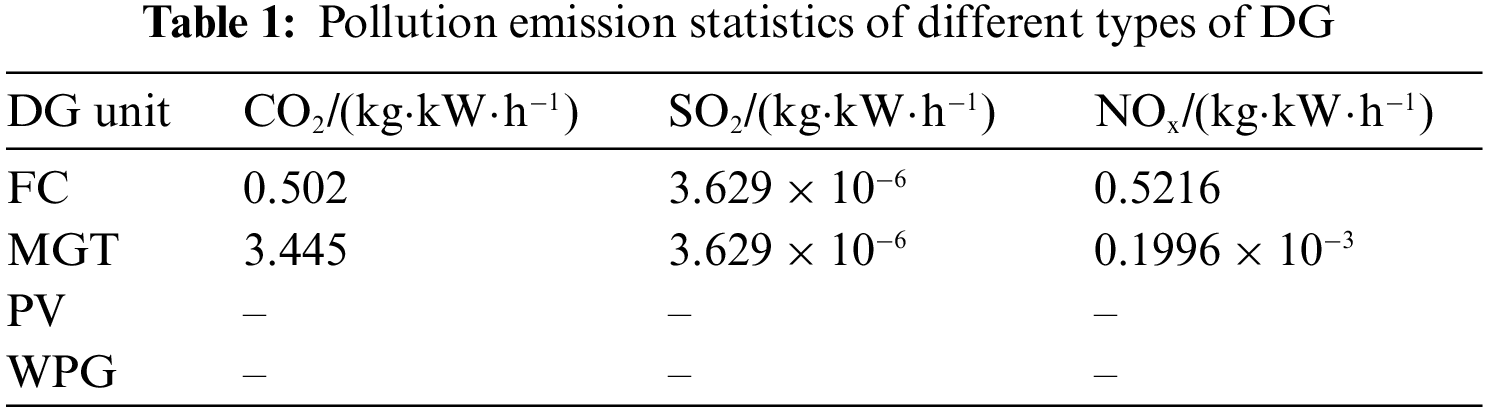
As can be seen from the above table, photovoltaic systems and wind turbines in addition to the construction period will produce pollution emissions, after the completion of power generation will not produce pollution emissions, belong to clean electricity. However, fuel cells and micro-gas turbines not only produce pollution emissions during construction, but also emit a certain amount of pollution emissions in the environment after the completion of power generation. Therefore, this paper takes the pollution emission index as one of the objective functions, to maximize environmental friendliness.

2.1.4 Meteorological Indicators

This paper proposes an objective function considering the annual average wind speed v¯w and annual average radiation intensity I¯S, to install wind turbines and photovoltaic systems in areas rich in wind and light resources to maximize the consumption of scenic energy, which can be expressed as follows:

minf6(x)=1∑anw1,av¯w,a+w2,aI¯S,a(11)

{w1,a=0,1w2,a=0,1(12)

where v¯w,a and I¯S,a are the annual average wind speed and the annual average radiation intensity at the a-th node, respectively; w1,a and w2,a are the weighting coefficients of wind and solar energy at the a-th node, respectively, which take the value of 0 or 1, and when the value of 1, it indicates that the a-th node is the siting point of DG. Notably, if w1,a and w2,a are both 1, it indicates that the a-th node is configured with wind-solar hybrid power generation system.

2.1.5 Distribution Network Tie-Line Exchange Power Deviation

Due to the intermittent nature of the new energy output, large power fluctuations will occur when it is connected to the grid. In this paper, the power stability of the grid is considered in the DG sizing and capacity planning, which is expressed in terms of the daily power deviation of the power tie-line as follows:

minf7(x)=∑t=1T[PTie-line(t)−P¯Tie-line]2(13)

where PTie-line(t) represents the switching power deviation of the Tie line of the grid at time t; P¯Tie-line indicates the average power exchange deviation in a day.

2.2 Constraints

(1) Transmission line power constraint.

|Sk|≤|Skmax|(14)

where Sk and Skmax represent the apparent power and maximum apparent power of the k-th node, respectively.

(2) Node voltage constraint.

VDG,kmin≤VDG,k≤VDG,kmax(15)

where VDG,kmin and VDG,kmax mean the upper and lower limits of the node voltage of node k after DG connection, respectively, which are 1.05 and 0.9 p.u.

(3) DG configuration power constraint.

PDG,imin≤PDG,i≤PDG,imin(16)

where PDG,imin and PDG,imin represent the upper and lower limits of the output power for the i-th DG unit.

(4) Node power balance.

{∑k=1NnodesPk−Ploss=∑k=1NnodesPload,k−∑k=1NnodesPDG,k∑k=1NnodesQk−Qloss=∑k=1NnodesQload,k−∑k=1NnodesQDG,k(17)

where Pk and Qk denote the active power and reactive power injected into node k, respectively; Ploss and Qloss mean the total active and reactive power losses in the system; Pload,k and Qload,k represent the active and reactive loads at node k; PDG,k and QDG,k represent the active and reactive power output of the DG unit connected at node k.

3  Design of Model Solver Based on MOABC-Improved Grey-Target Decision-Making

3.1 Artificial Bee Colony Algorithm

Let ABC be presented as a multi-objective intelligent optimization algorithm to mimic the process of bees collecting nectar in nature. It consists of a food source, leading bees, and follower bees. The solution process is as follows:

(1) The population is initialized based on upper and lower limits, followed by the calculation of initial fitness function values.

(2) The leading bees will continuously update their food sources to ensure the freshness of their food. After updating the food source, bees will update the fitness values and optimal food source according to the new food source. The process of updating the food source is as follows:

newij=a+b×foodij(18)

a=c1×foodij+(1−c1)×gbestj(19)

b=|foodij−gbestj|(20)

where foodij represents the j-th food obtained by the i-th population, gbest is the best food source of the current population, and c1 is a random number in [0,1].

(3) After updating the food source, the leading bees will share information with the follower bees. The follower bees will then allocate to the food sources.

(4) The bee colony will allocate food based on the information provided by the follower bees, which can be calculated as

newij=rand(0,1)×(ref1,i−ref2,i)(21)

where ref1,i and ref2,i are two reference foods selected from the previous foods, and rand is a randomly generated new food source within the constraint range.

(5) If the food source falls into a local optimum, it will be abandoned. The scout bees will then generate a new food source based on Eq. (18), which can be calculated as

newij=rand(lb,ub)(22)

where lb and ub are the upper and lower limits of the decision variables. Similar to step 2, the bees will update the fitness values and the optimal food source.

(6) Repeat steps (2) to (5) until the end of the cycle to obtain the optimal food source and fitness value.

3.2 Multi-Objective Artificial Bee Colony Algorithm

Multi-objective optimization problems are different from single-objective ones, as it is impossible to obtain a solution that minimizes all objectives at the same time, only a set of Pareto optimal solutions can be obtained [18]. The flowchart of MOABC is shown in Fig. 1. This section introduces the selection mechanism of MOABC, as follows:

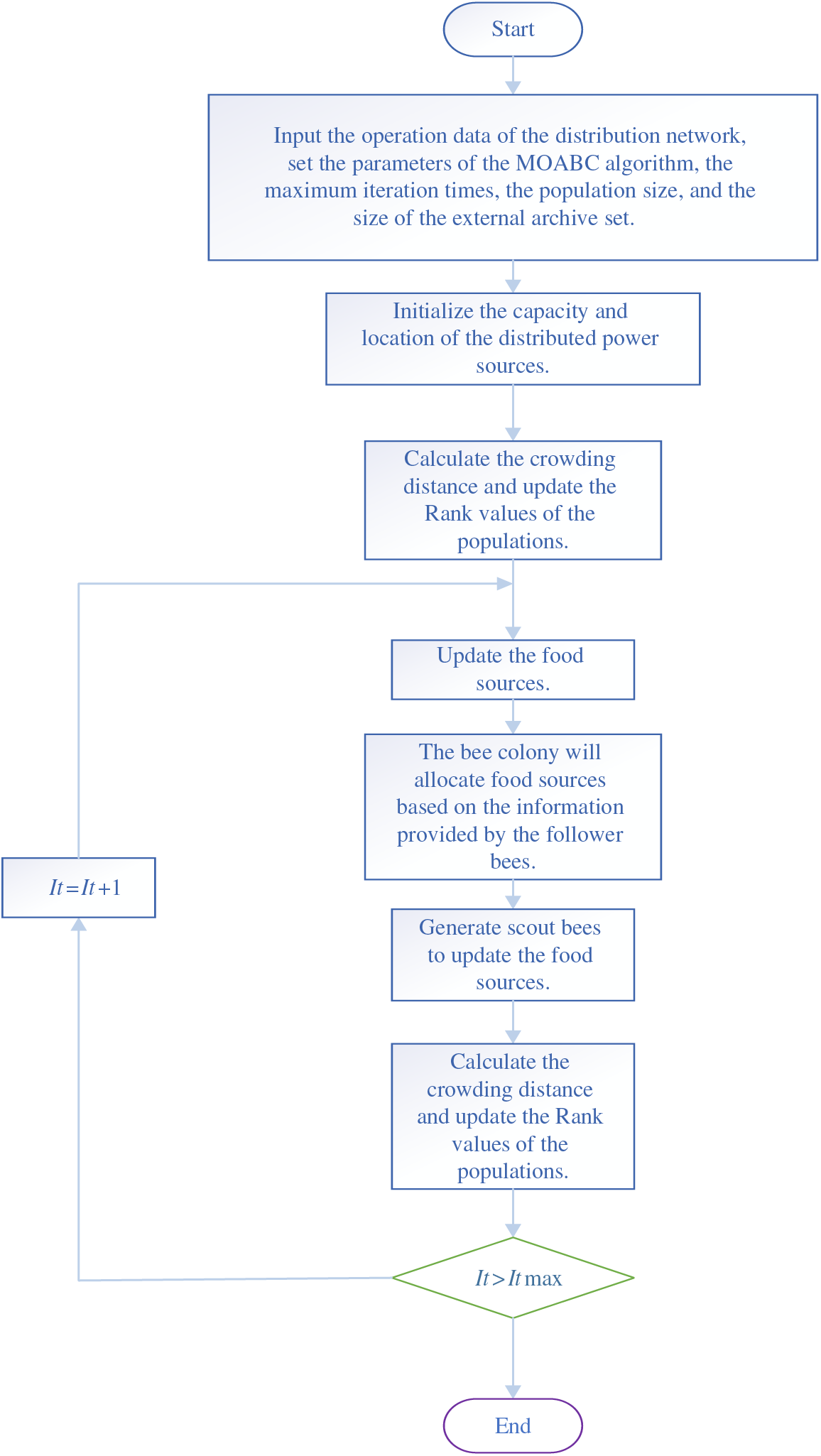
Figure 1: The flowchart of location and capacity selection of DG based on MOABC

(1) An external archive is added to MOABC to store non-dominated solutions, with capacity limited to a fixed number.

(2) A solution update mechanism based on Pareto non-dominated ranking.

(3) Calculate the crowding distance of all populations, and rank populations with the same level based on the size of the crowding distance.

3.3 Improved Grey-Target Decision-Making

In order to avoid the influence of subjective decision on the final result, the grey target decision scheme based on the entropy weight method (EWM) [19] is adopted in this study, and the compromise solution of the Pareto non-dominated solution set is taken as the optimal decision scheme. Firstly, the sample matrix is established based on the Euclidean distance and Mahalanobis distance between the normalized Pareto solution set and each solution set. Secondly, the decision matrix [20] is established according to the cost index formula, and then the bull’s-eye is selected in the gray area formed by the decision matrix. Finally, the weight and entropy of each group of solutions are calculated, and the distance between each group of solutions and the bullseye is calculated based on the weight and entropy. The solution closest to the bull’s eye is selected as the best compromise [21].

(1) Build a sample matrix

The normalized fitness function F of all the solutions is taken as one of the evaluation indexes, and the sample matrix is established. In this paper, we consider adding two related indexes to the sample matrix, one is the Euclidean distance (ED) ED between each solution and the ideal point, and the other is the Mahalanobis distance (MD) MD between each solution and the equilibrium point. So the sample matrix is represented by:

x=[F,ED,MD]=(xao)n′×(m′+2)=[F11⋅sFm′1ED1MD1F12⋅sFm′2ED2MD2⋮⋅s⋮⋮⋮F1n′⋅sFm′n′EDn′MDn′](23)

Fao=(Famax−Famin)(fao−famin)(famax−famin)+Famin(24)

EDo=∑a=1m′+2(Fao−Oa)2(25)

MDo=∑a=1m′+2(Fao−ua)T∑−1(Fao−ua)(26)

In the formula, n′ prime and m′ primes are the number of objective functions and the number of settlements, respectively; fao is the a-th fitness function of the o-th solution; famin and famax are the maximum and minimum fit values of the a-th objective function, respectively. Fao is the a-th fitness function of the o-th solution after normalization. Oa is the ideal point of the a-th objective function. ua is the mean of the a-th objective function. ∑−1 is the covariance matrix.

(2) Computational bullseye

The operator qa is used to dimensionalize the sample matrix, and its calculation formula is as follows:

qa=1n′∑o=1n′(xao),a=1,2⋯,m′+2(27)

where xao is the evaluation index of the o goal of the a solution.

The decision matrix V is established based on the operator qa and the sample matrix, as follows:

V=(vao)n′×(m′+2)=qa−xaomax{max1≤o≤n′{xao}−qa−min1≤o≤n′{xao}}(28)

The selected bullseye is vao=min{vao|1≤o≤n′}.

(3) Establish the weight and Mahalanobis distance

Based on EWM, the weights of each evaluation index can be obtained objectively, and the optimal compromise solution can be selected from Pareto non-dominated solution set. The weights ωa and entropy Ea are calculated as follows:

ωao=xao/∑o=1n′(xao),xao≫0(29)

Ea=−1ln⁡n′∑o=1n′(ωaoln⁡ωao),Ea>0(30)

ωa=(1−Ea)/∑a=1m′+2(1−Ea)(31)

Each MD to the bullseye can be expressed as:

Mo=|vo−v0|=∑a=1m′+2ωa(Fao−ua)T∑−1(Fao−ua)(32)

The non-dominated solutions are sorted according to MD. Each set of solutions in the archive set is considered an independent decision scheme. The solution closest to the bullseye is chosen as the optimal decision solution.

4  Case Studies

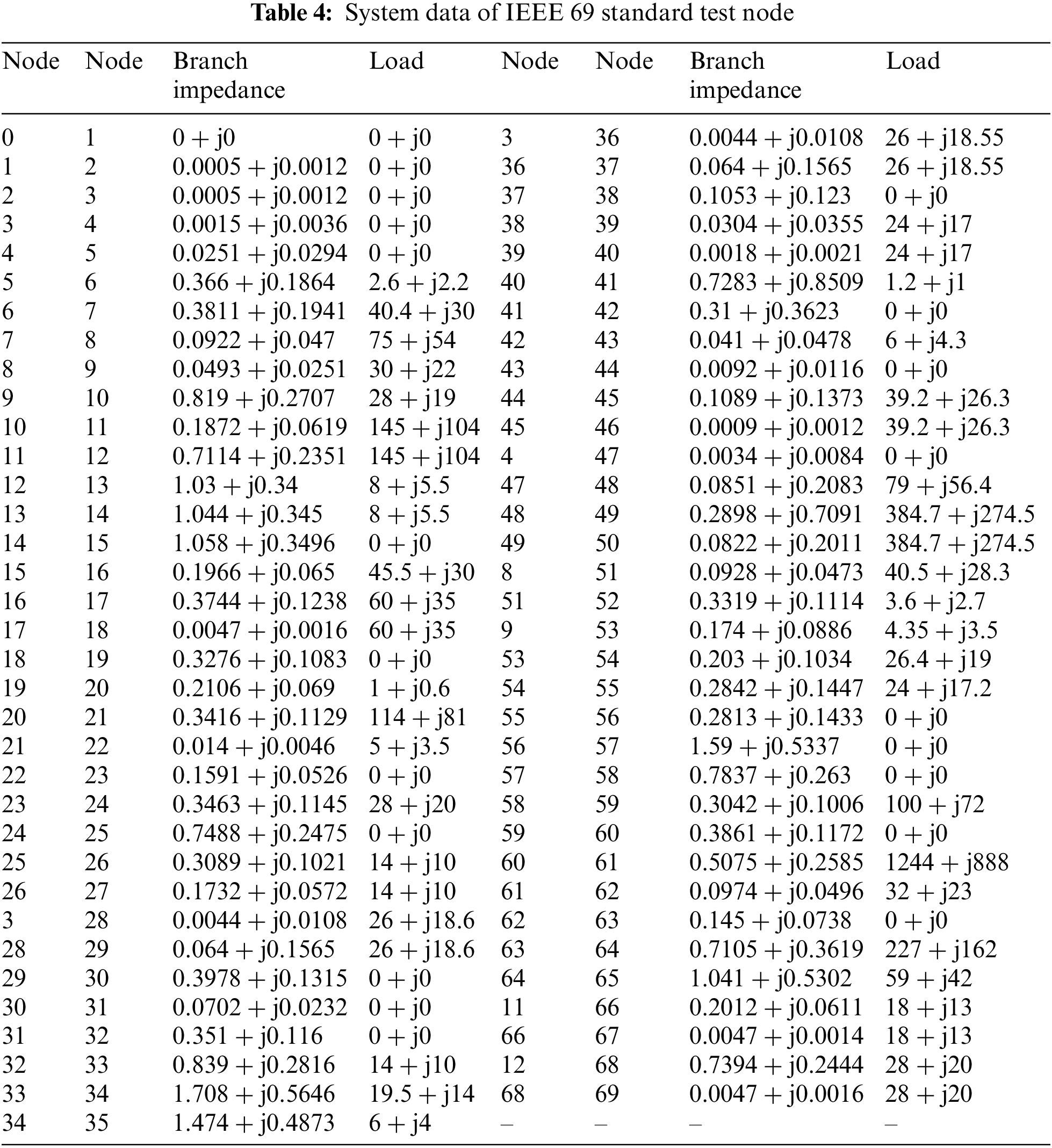
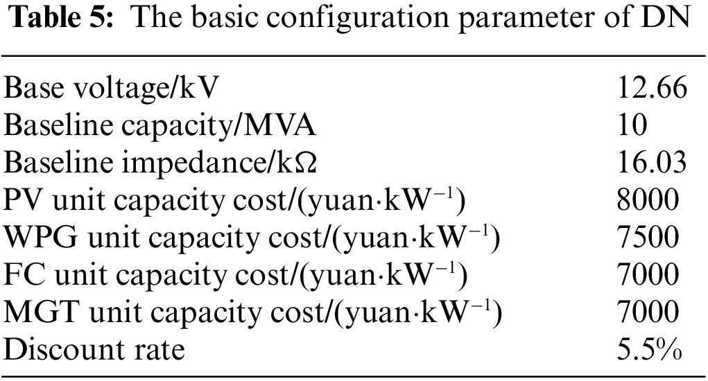
In order to verify the effectiveness of the multi-objective optimization algorithm proposed in this paper [22], a DG siting constant volume simulation test based on IEEE 33 and IEEE 69 standard test node system was designed, and two PV, two WPG, one FC and one MGT were configured. In addition, the optimization results of MOABC were compared with MODA, MOGOA and MOPSO. In order to ensure the fairness of algorithm comparison, the maximum number of iterations and population of the two algorithms were set to 100 and 100, respectively [23]. In addition, the simulation tests of all the examples were completed in MATLAB 2022a environment on a computer equipped with Intel (R) Core (TM) i9-13900K 3.0 GHz CPU and 128 GB memory. Table 2 shows the statistical table of the control parameters of the MOABC algorithm, and Fig. 2 shows the topology structure of the IEEE 33 standard test node system. Table 3 shows the system data of IEEE 33 standard test node [24]. Fig. 3 shows the system topology structure of IEEE 69 standard test nodes, Table 4 shows the system data of IEEE 69 standard test nodes, and Table 4 shows the basic configuration parameters of DN. The basic configuration parameters of DN and the cost parameters of DG are given in Table 5.

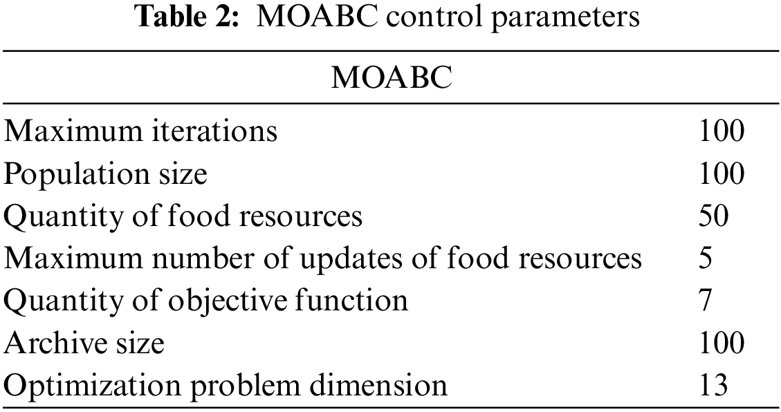
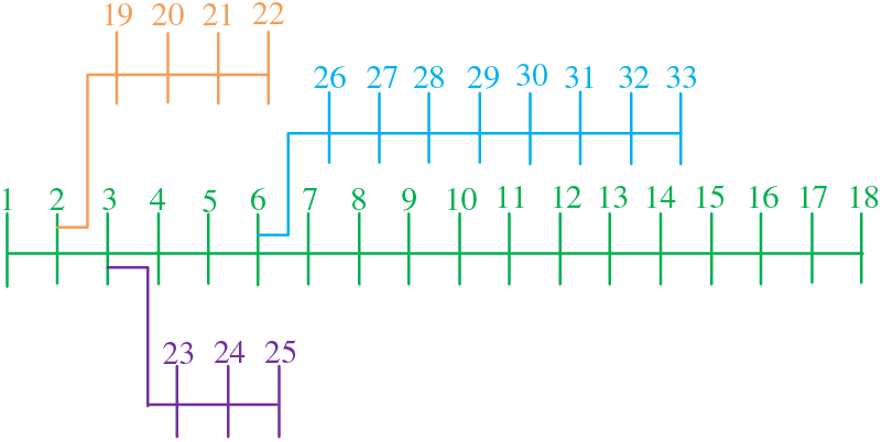
Figure 2: Topology of IEEE 33 standard test nodes system

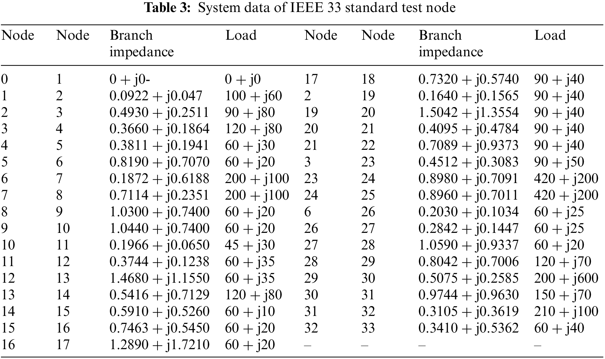
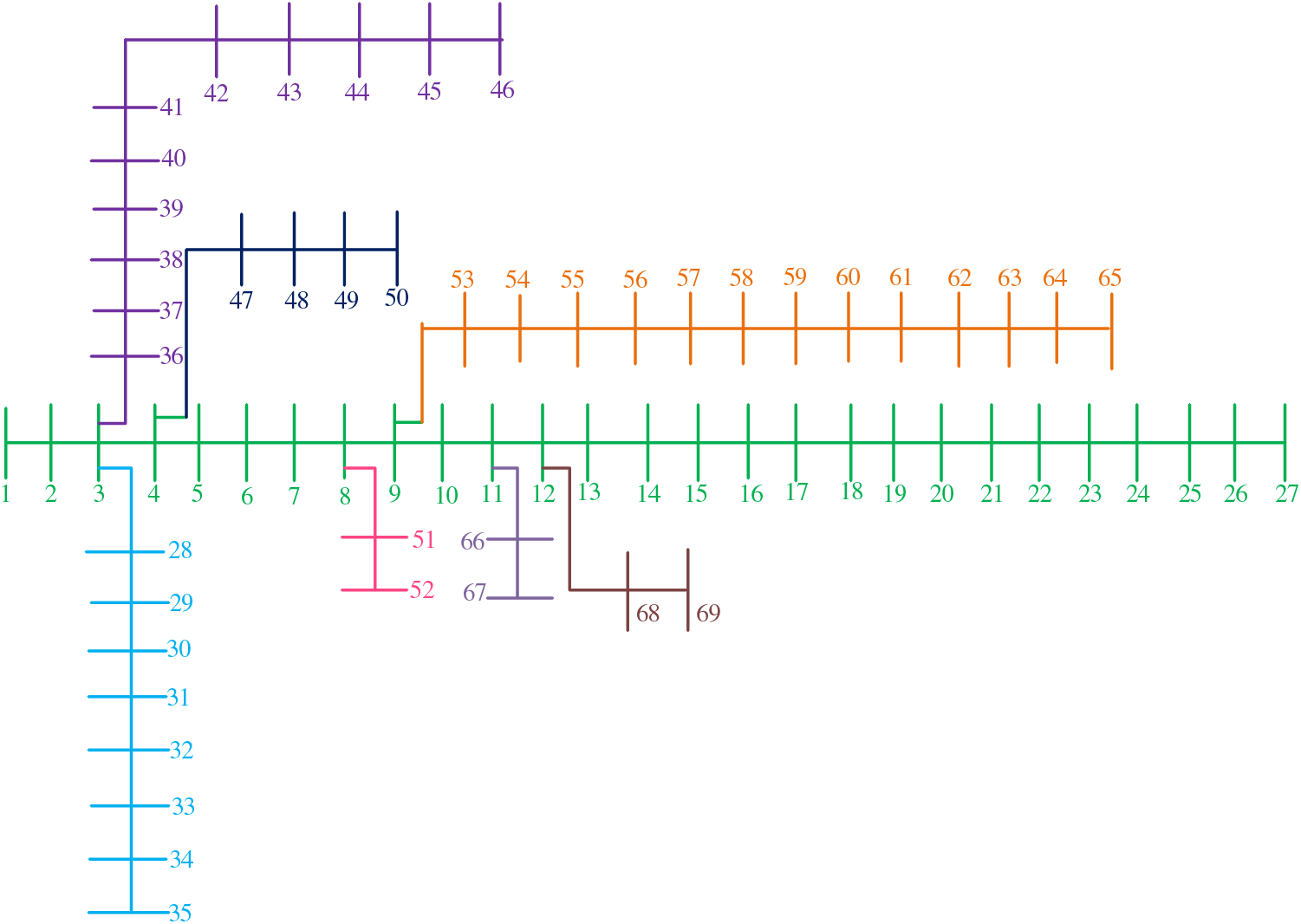
Figure 3: Topology of IEEE 69 standard test nodes system

The MOABC control parameters in the table above are most consistent with the research topic of this paper.

4.1 Performance Comparison of IEEE 33 Node Algorithm

Table 6 shows the upper and lower limits of DG capacity constraints. Table 7 shows the specific configuration schemes of four types of DG obtained by MOABC. Table 8 shows the optimization results of configuring DG in the IEEE 33 node test system via MOABC, MODA, MOGOA and MOPSO, respectively. Compared with no DG configuration, MOABC algorithm costs $3.473×104 after DG configuration. The total voltage deviation, voltage fluctuation, system network loss and tie-line power deviation of DN decreased by 32.88 p.u (49.67%), 0.082 p.u (7.47%), 1954.77 kW (48.12%) and 71.33 kW (5.90%), respectively, among the 7 objective functions, MOABC can obtain the optimal results in the 5 targets of total voltage deviation, voltage fluctuation, system network loss, power deviation of the liaison line and weight of meteorological indicators. This shows that the results obtained by MOABC are friendly to users and power grid companies, and are only $0.957×104 higher than MOPSO, which has the lowest configuration cost. The pollution emission coefficient of 151.29 kg/h obtained by MOABC is only lower than MOPSO, and compared with the optimized results of MODA and MOGOA, this result has certain environmental friendliness. In addition, the weight of the meteorological index of MOABC configuration scheme is 0.8188, which is close to 1, indicating that the PV and WPG position configured in this scheme can make better use of natural scenery resources and effectively improve the utilization rate of scenery resources.

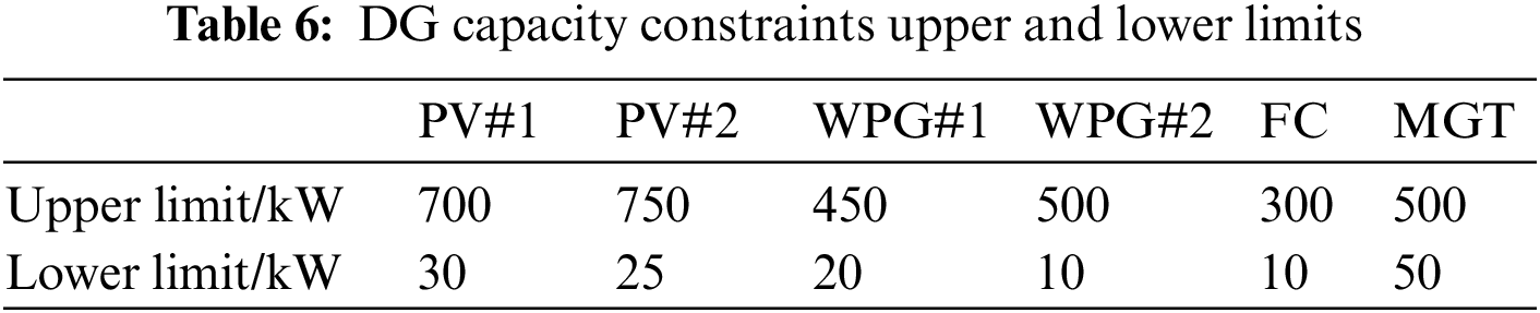
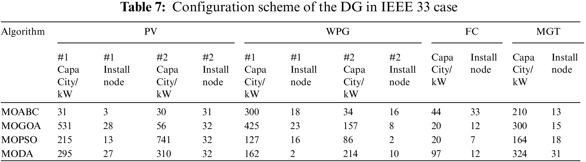
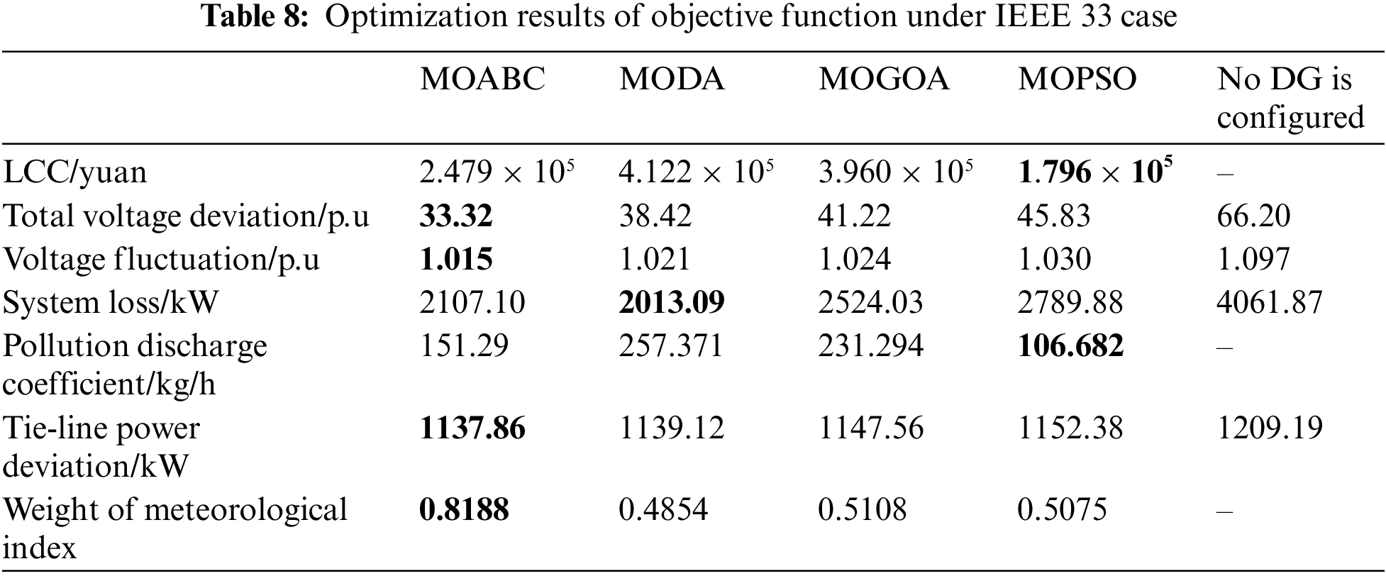
Fig. 4 shows the box plot drawn by each algorithm after 10 independent runs under the same number of iterations, population number and constraints. As can be seen from the figure, among the seven objective functions of MOABC compared with other algorithms, four have good stability and all have good numerical performance, indicating that MOABC has the best stability and effectiveness among the four algorithms.

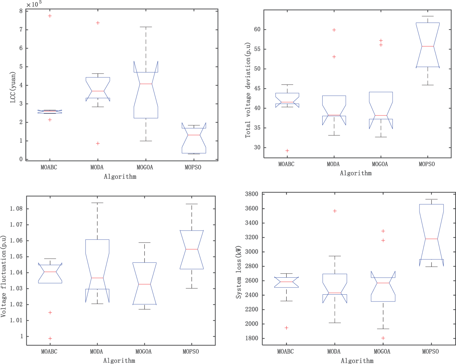
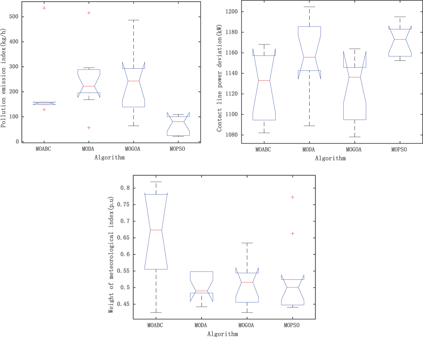
Figure 4: Target function box plot of each algorithm (IEEE 33)

Figs. 5 and 6 respectively show the voltage fluctuation diagram of DN after DG configuration with MOABC and the voltage level distribution diagram of 33 nodes. As can be seen from the figure, the node voltage level of 33 nodes increases after DG is configured, which is closer to 1 p.u. This shows that compared with MODA, MOGOA and MOPSO, the DG configuration scheme selected by MOABC can effectively improve the stability of DN operation and give full play to the positive role of DG in DN.

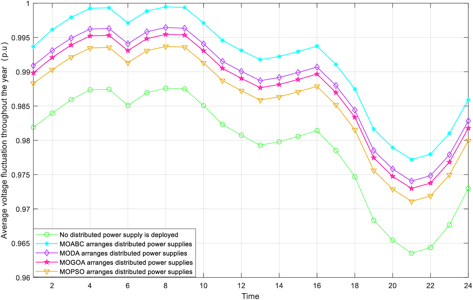
Figure 5: Comparison of the voltage fluctuation curves of DN before and after the configuration of DG at node 33

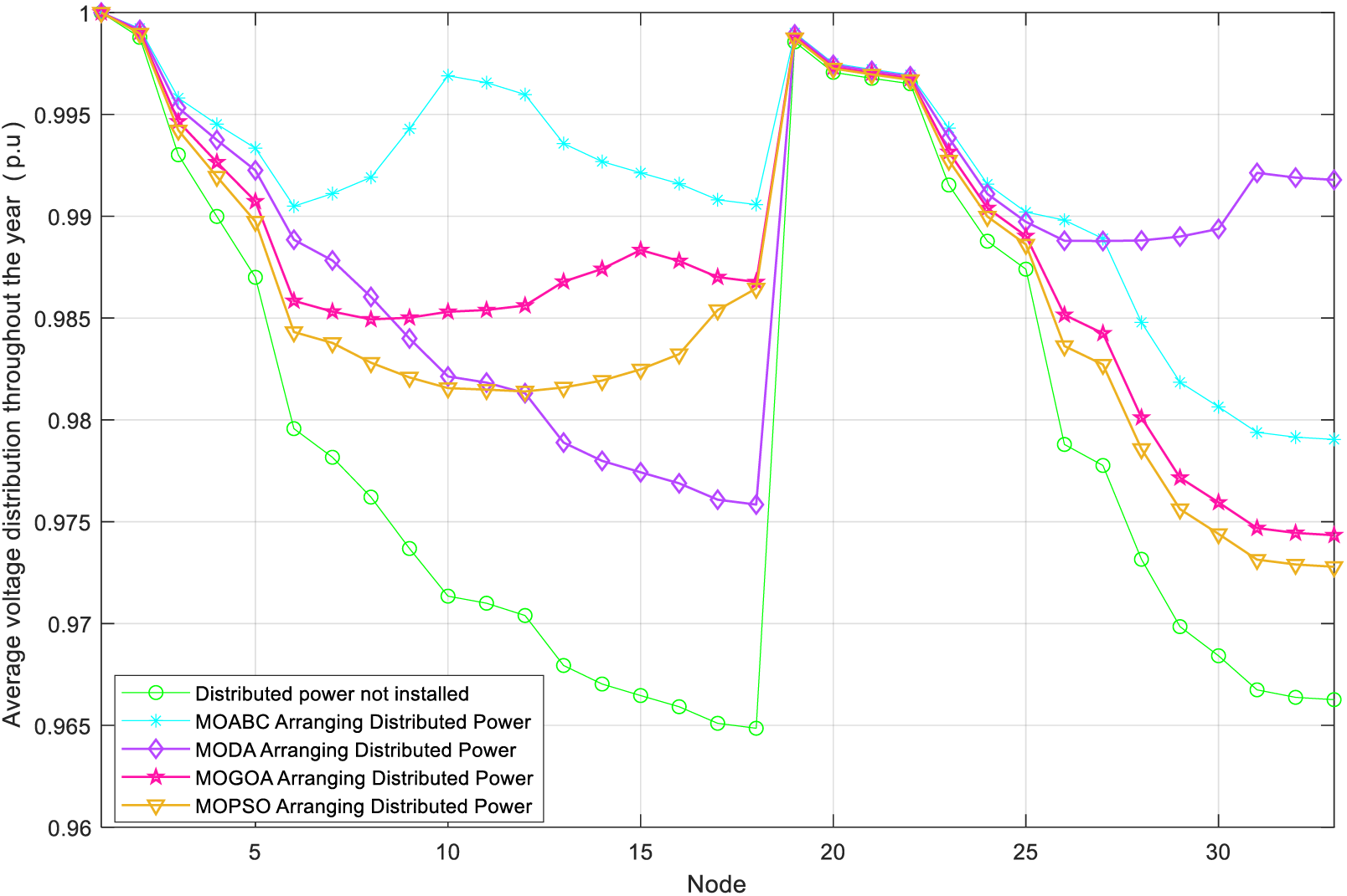
Figure 6: Comparison of node voltage levels of DN before and after configuration of DG at 33 nodes

4.2 Performance Comparison of IEEE 69 Node Algorithm

Table 9 shows the specific configuration schemes of the four DGs obtained by MOABC. Table 10 gives the optimization results of configuring the DG in the IEEE 69-node test system via MOABC, MODA, MOGOA and MOPSO, respectively. Compared to the unconfigured DG, the MOABC algorithm spends $3.392×104 to configure the DG, the total voltage deviation, voltage fluctuation in terms of, system network loss and tie-line power deviation of the DN decreases by 39.25 p.u (54.98%), 0.425 p.u (35.93%), 3345.22 MW (75.17%) and 424.135 kW (33.91%). By comparing the optimization results of each algorithm in Table 9, MOABC can obtain optimal results in five objectives among seven objective functions: total voltage deviation, voltage fluctuation, system network loss, power deviation of the tie-line and weight of meteorological indicators. This indicates that MOABC is able to obtain results that are user and grid company friendly. In addition, the meteorological indicator weight of the MOABC configuration scheme is 0.8180, which is close to 1. This indicates that the PV and WPG locations configured in this scheme can better utilize the natural scenic resources and effectively improve the utilization rate of scenic resources.

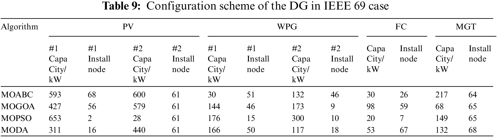
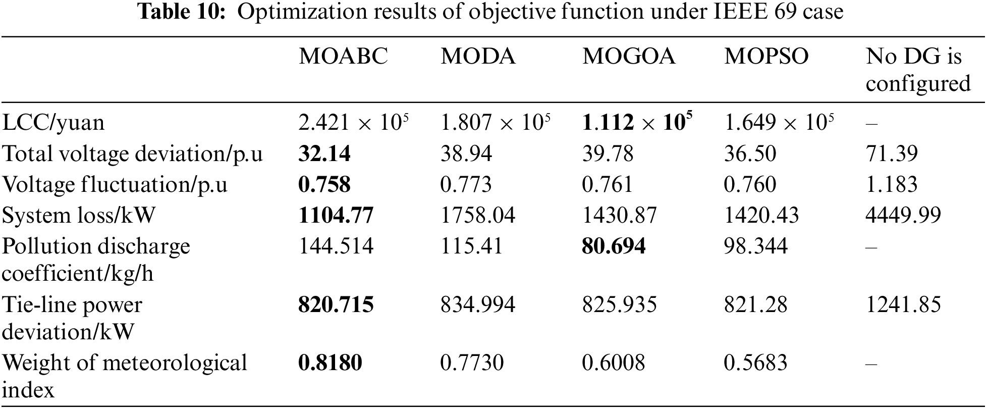
Fig. 7 shows the box plots of each algorithm after 10 independent runs with the same number of iterations, population size and constraints. From the figure, it can be seen that MOABC has good stability and good numerical performance in six of the seven objective functions compared with other algorithms, indicating that MOABC has the best stability and effectiveness among the four algorithms.

Figure 7: Target function box plot of each algorithm (IEEE 69)

Figs. 8 and 9 show the voltage fluctuation graph of DN after MOABC configured DG and the distribution of node voltage level of 69 nodes, respectively. From the figures, it can be seen that the node voltage levels of the 69 nodes after configuring the DG have increased and are closer to 1 p.u. This shows that the DG configuration scheme that MOABC can select can effectively improve the stability of DN operation compared to the schemes of MODA, MOGOA and MOPSO, and can fully utilize the positive role of DG in DN.

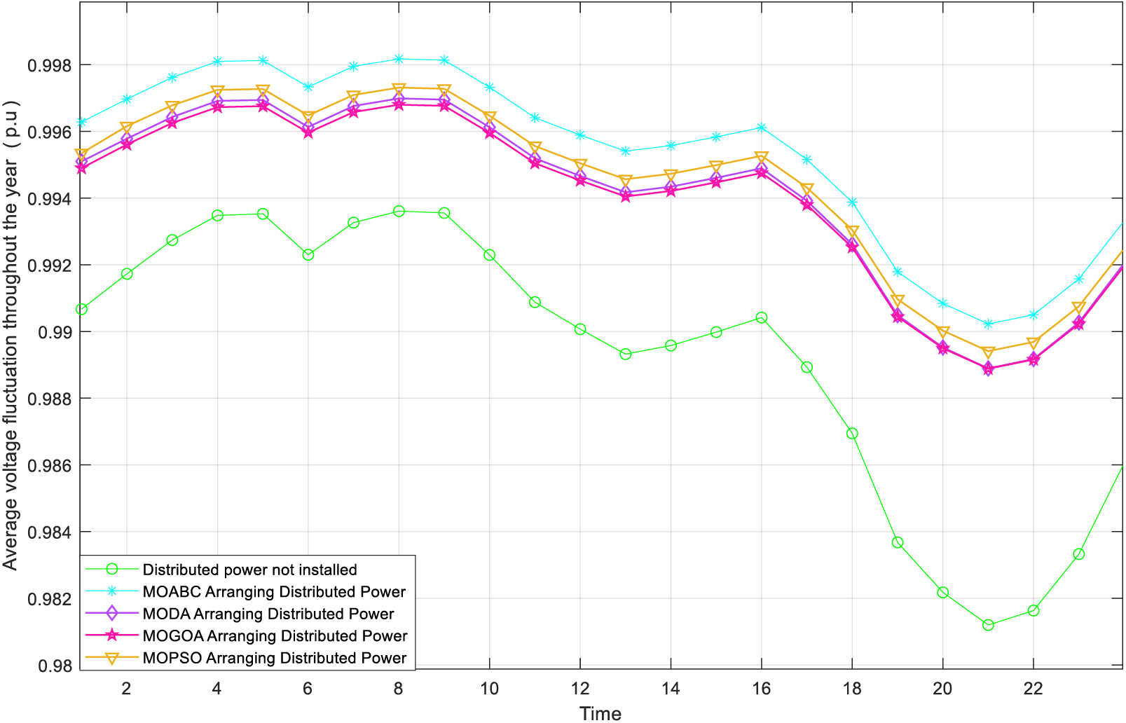
Figure 8: Comparison of the voltage fluctuation curves of DN before and after the configuration of DG at node 69

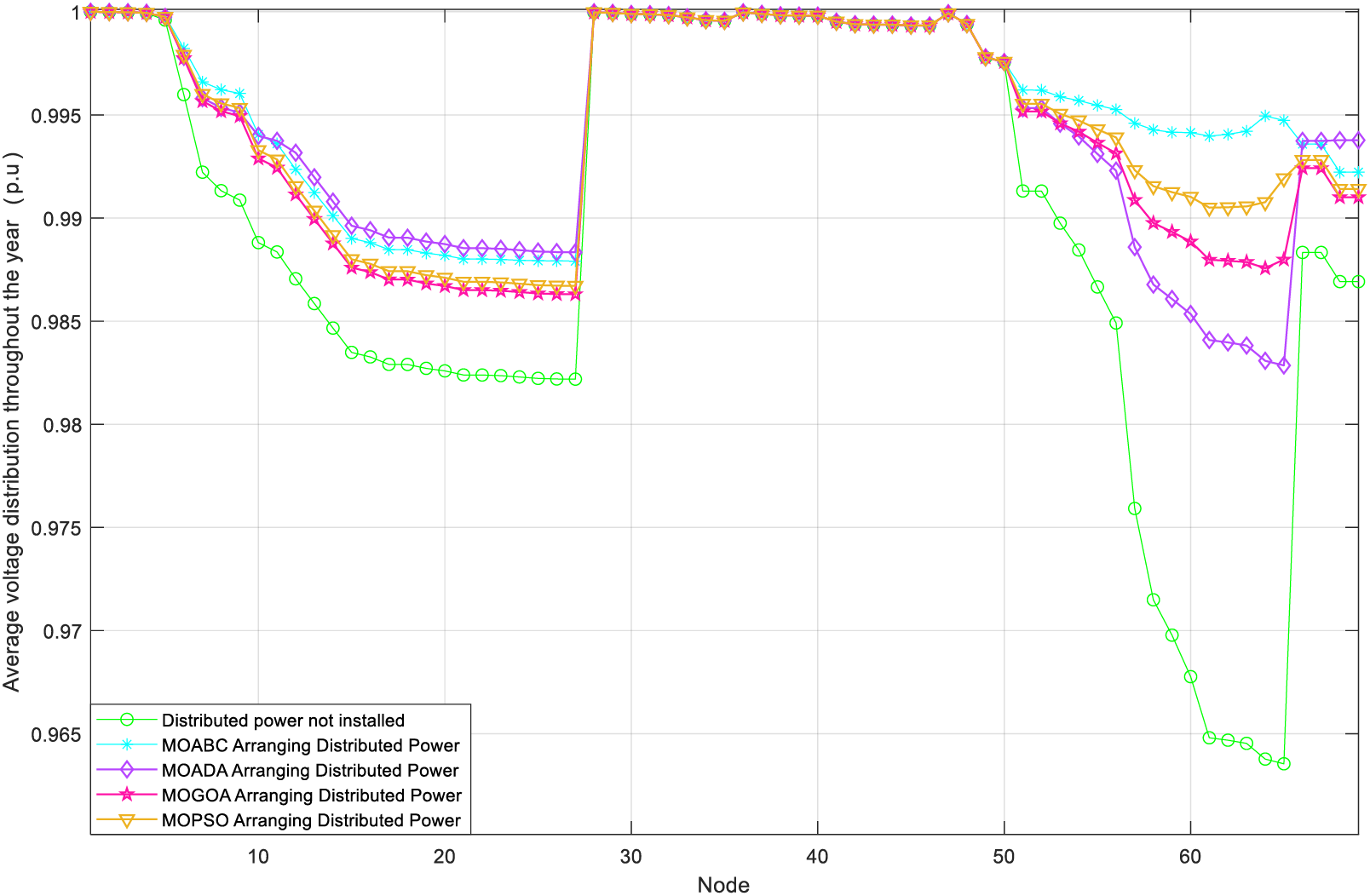
Figure 9: Comparison of node voltage levels of DN before and after configuration of DG at 69 nodes

5  Conclusion

Considering the operation stability of DN, the investment economy of DG, the environmental friendliness and the full utilization of scenic resources, this paper carries out the capacity allocation location of four typical DG based on MOABC. Based on the improved grey target decision, the optimal compromise solution is obtained. The main conclusions are as follows:

1) This paper establishes a multi-objective programming model based on DG LCC, pollution emission index, meteorological index weight and DN voltage fluctuation, voltage distribution, network loss and tie-line power deviation. It can achieve the maximum improvement of DN stability and economy on the premise of ensuring the interests of DG investors.

2) In this paper, an improved grey target decision scheme based on Euclidean distance and Mahalanobis distance is adopted, which can effectively avoid the influence of subjective decision on the optimal compromise solution.

3) In this paper, a simulation experiment based on IEEE 33 standard node test system is designed to verify the validity of the proposed configuration method. The experimental results show that the total voltage deviation, voltage fluctuation and system network loss of DN decreased by 49.67%, 7.47% and 48.12% respectively after the DG configured by MOABC. The stability of DN operation is effectively improved.

4) In this paper, a simulation experiment based on IEEE 69 standard node test system is designed to verify the validity of the proposed configuration method. The experimental results show that the total voltage deviation, voltage fluctuation and system network loss of DN decreased by 54.98%, 35.93% and 75.17% respectively after the DG configured by MOABC. The stability of DN operation is effectively improved.

In this paper, based on IEEE 33 and IEEE 69 distribution network structure, MOABC is used to locate and determine the capacity of four types of DG. After the optimized configuration of DG is connected to DN, the total voltage deviation and voltage fluctuation of DN are significantly reduced, which is conducive to the more stable and economical operation of DN. It shows that the distribution of distributed generation is crucial to the success of grid planning [25]. At the same time, compared with other schemes, the configuration scheme of MOABC has the smallest configuration capacity, but can improve the stability and economy of DN to the greatest extent, and the configuration scheme is more effective. Secondly, the configuration scheme of MOABC can maximize the utilization of scenery resources and has good economic and environmental protection, and its configuration scheme has better economy, environmental protection and high efficiency. Finally, MOABC has better stability and effectiveness compared to MODA, MOGOA and MOPSO, as shown in the box whisker diagram.

Acknowledgement: Thank you very much for the support provided by State Grid Shaanxi Electric Power Company and Central Southern China Electric Power Design for this paper.

Funding Statement: The authors received no specific funding for this study.

Author Contributions: Qiangfei Cao: Conceptualization, Writing-reviewing, and editing; Huilai Wang: Writing-original draft preparation, Investigation; Zijia Hui: Visualization and contribution to the discussion of the topic; Lingyun Chen: Validation.

Availability of Data and Materials: All data are from a region in Southwest China, and the data used cannot be disclosed according to data confidentiality requirements.

Conflicts of Interest: The authors declare that they have no conflicts of interest to report regarding the present study.

References

1. Li, G. D., Wang, Z., Zhao, F. Z., Hao, S., Zhang, Q. C. et al. (2021). Evaluation of the impact of distributed generation access on distribution network operation index. Electrical and Energy Management Technology, 603(6), 79–85. [Google Scholar]

2. Song, D. R., Liang, Z. A., Xia, E., Yang, J., Liu, J. B. et al. (2023). Overview of wind power life-cycle cost modeling and economic analysis. Thermal Power Generation, 52(3), 1–12. [Google Scholar]

3. Jiao, Y. L., Fan, X. C., Shi, R. J., Wang, W. Q., Liu, S. M. et al. (2022). Optimal configuration of AC/DC hybrid microgrid based on GTMPSO algorithm. Journal of Kunming University of Science and Technology (Natural Science), 47(4), 72–82. [Google Scholar]

4. Yang, B., Wang, J. T., Chen, Y. X., Li, D. Y., Zeng, C. Y. et al. (2020). Optimal sizing and placement of energy storage system in power grids: A state-of-the-art one-stop handbook. Journal of Energy Storage, 32, 101814. [Google Scholar]

5. Wei, W., Fan, Y., Xie, R., Bai, J. Y., Mei, S. W. (2023). Optimal ratio of wind-solar-storage capacity for mitigating the power fluctuations in power system with high penetration of renewable energy power generation. Electric Power Construction, 44(3), 138–147. [Google Scholar]

6. Wang, X., Chen, Z. C., Bian, Z. H., Wang, Y. Y., Wu, Y. M. (2022). Optimal allocation of a wind−PV−battery hybrid system in smart microgrid based on particle swarm optimization algorithm. Integrated Intelligent Energy, 44(6), 52–58. [Google Scholar]

7. Quadri, I. A., Bhowmick, S., Joshi, D. (2019). A hybrid teaching-learning-based optimization technique for optimal DG sizing and placement in radial distribution systems. Soft Computing, 23(20), 9899–9917. [Google Scholar]

8. Boktor, C. G., Youssef, A. R., Kamel, S. (2019). Optimal installation of renewable DG units in distribution system using hybrid optimization technique. IEEE Conference on Power Electronics and Renewable Energy (IEEE CPERE), pp. 129–134. Aswan, Egypt. [Google Scholar]

9. Zhang, X. J., Kong, D. H., Ma, Q. L., Sun, Z. (2023). Research on distributed generation access method based on line loss optimization. Electric Engineering, 590(8), 226–229. [Google Scholar]

10. Liu, K., Liu, D. P., Guo, C., Wang, X., Zhang, Q. S. et al. (2022). DG site selection and capacity planning method in distribution network based on BFOA algorithm. Power Grid Analysis & Study, 50(9), 90–96. [Google Scholar]

11. Yang, Y., Wang, T. (2022). Optimal siting and sizing of distributed generators based on multi-objective double-layer planning. Journal of North China Electric Power University (Natural Science Edition)(In Chinese). http://kns.cnki.net/kcms/detail/13.1212.TM.20220803.1152.002.html [Google Scholar]

12. Yang, B., Yu, L., Chen, Y. X., Ye, H. Y., Shao, R. N. et al. (2021). Modelling, applications, and evaluations of optimal sizing and placement of distributed generations: A critical state-of-the-art survey. International Journal of Energy Research, 45(3), 3615–3642. [Google Scholar]

13. Abdel-Mawgoud, H., Kamel, S., Ebeed, M., Aly, M. M. et al. (2018). An efficient hybrid approach for optimal allocation of DG in radial distribution networks. International Conference on Innovative Trends in Computer Engineering (ITCE), pp. 311–316. Aswan, Egypt. [Google Scholar]

14. Ramadan, A., Ebeed, M., Kamel, S., Ahmed, E. M., Tostado-Veliz, M. et al. (2023). Optimal allocation of renewable DGs using artificial hummingbird algorithm under uncertainty conditions. Ain Shams Engineering Journal, 14(2), 101872. [Google Scholar]

15. Yang, B., Li, J. L., Li, Y. L., Guo, Z. X., Zeng, K. D. et al. (2022). A critical survey of proton exchange membrane fuel cell system control: Summaries, advances, and perspectives. International Journal of Hydrogen Energy, 47(17), 9986–10020. [Google Scholar]

16. Zheng, J. L., Chen, J., Zhao, L. H., Yang, G., Yu, L. (2022). Research progress of life cycle cost technology in domestic power system. Electric Engineering, 563(5), 37–41. [Google Scholar]

17. Wu, X. M., Shi, Z., Fu, Z. Y., Liu, X. Y., Dang, J. et al. (2022). Multi-scene distributed generation planning based on clustering by fast search and find of density peak. Journal of Henan Polytechnic University (Natural Science), 41(2), 117–123. [Google Scholar]

18. Zhang, Y. (2023). MOABC for CSFS. https://www.mathworks.com/matlabcentral/fileexchange/71151-moabc-for-csfs [Google Scholar]

19. Fang, T., Jiang, D., Yang, Y., Yuan, T. J. (2022). Research on business operation mode of hydrogen integrated energy system based on NSGA-II and entropy weight method. Electric Power, 55(1), 110–118. [Google Scholar]

20. Yang, H. H., Wang, J., Tai, N. L., Ding, Y. T. (2019). Robust optimization of distributed generation in a microgrid based on grey target decision-making and multi-objective cuckoo search algorithm. Power System Protection and Control, 47(1), 20–27. [Google Scholar]

21. Zhang, C., Zhou, J., Zhao, B., Li, J. L., Yang, B. (2022). Multi-objective optimal configuration of electricity-hydrogen hybrid energy storage system in zero-carbon park. Electric Power Construction, 43(8), 1–12. [Google Scholar]

22. Wang, H. M., Yang, P., Yu, Y. L. (2021). Optimal distributed generation planning in active distribution network based on Bi-level particle swarm optimization algorithm. Computer & Digital Engineering, 49(9), 1930–1935. [Google Scholar]

23. Jeong, Y. C., Lee, E. B., Alleman, D. (2019). Reducing voltage volatility with step voltage regulators: A life-cycle cost analysis of Korean solar photovoltaic distributed generation. Energies, 12(4), 652. [Google Scholar]

24. Zakeri, B., Syri, S. (2016). Electrical energy storage systems: A comparative life cycle cost analysis. Renewable and Sustainable Energy Reviews, 53, 1634–1635. [Google Scholar]

25. Pereira, L. D. L., Yahyaoui, I., Fiorotti, R., de Menenzes, L. S., Fardin, J. F. et al. (2022). Optimal allocation of distributed generation and capacitor banks using probabilistic generation models with correlations. Applied Energy, 307(3), 118097. [Google Scholar]