
 Submit a Paper
 Propose a Special lssue
 Open Access
ARTICLE

Performance Analysis of Various Forecasting Models for Multi-Seasonal Global Horizontal Irradiance Forecasting Using the India Region Dataset
Department of Business Development and Technology, Aarhus School of Business and Social Sciences (BSS), Aarhus University, Birk Centerpark 15, Herning, 7400, Denmark
* Corresponding Authors: Manoharan Madhiarasan. Email: or
(This article belongs to the Special Issue: Innovative Energy Engineering for Resilient and Green Systems)
Energy Engineering 2025, 122(8), 2993-3011. https://doi.org/10.32604/ee.2025.068358
Received 27 May 2025; Accepted 26 June 2025; Issue published 24 July 2025
 View Full Text
 Download PDF
Abstract
Accurate Global Horizontal Irradiance (GHI) forecasting has become vital for successfully integrating solar energy into the electrical grid because of the expanding demand for green power and the worldwide shift favouring green energy resources. Particularly considering the implications of the aggressive GHG emission targets, accurate GHI forecasting has become vital for developing, designing, and operational managing solar energy systems. This research presented the core concepts of modelling and performance analysis of the application of various forecasting models such as ARIMA (Autoregressive Integrated Moving Average), Elaman NN (Elman Neural Network), RBFN (Radial Basis Function Neural Network), SVM (Support Vector Machine), LSTM (Long Short-Term Memory), Persistent, BPN (Back Propagation Neural Network), MLP (Multilayer Perceptron Neural Network), RF (Random Forest), and XGBoost (eXtreme Gradient Boosting) for assessing multi-seasonal forecasting of GHI. Used the India region data to evaluate the models’ performance and forecasting ability. Research using forecasting models for seasonal Global Horizontal Irradiance (GHI) forecasting in winter, spring, summer, monsoon, and autumn. Substantiated performance effectiveness through evaluation metrics, such as Mean Absolute Error (MAE), Root Mean Squared Error (RMSE), and R-squared (R2), coded using Python programming. The performance experimentation analysis inferred that the most accurate forecasts in all the seasons compared to the other forecasting models the Random Forest and eXtreme Gradient Boosting, are the superior and competing models that yield Winter season-based forecasting XGBoost is the best forecasting model with MAE: 1.6325, RMSE: 4.8338, and R2: 0.9998. Spring season-based forecasting XGBoost is the best forecasting model with MAE: 2.599599, RMSE: 5.58539, and R2: 0.999784. Summer season-based forecasting RF is the best forecasting model with MAE: 1.03843, RMSE: 2.116325, and R2: 0.999967. Monsoon season-based forecasting RF is the best forecasting model with MAE: 0.892385, RMSE: 2.417587, and R2: 0.999942. Autumn season-based forecasting RF is the best forecasting model with MAE: 0.810462, RMSE: 1.928215, and R2: 0.999958. Based on seasonal variations and computing constraints, the findings enable energy system operators to make helpful recommendations for choosing the most effective forecasting models.Keywords
Over the past two decades, solar energy systems have seen a rise in interest in renewable energy sources due to global warming and the energy shortage [1]. Several nations have strongly promoted solar energy as an environmentally friendly form of energy. India has an immense future for solar energy. Around 5000 trillion kWh of energy is catastrophe over India’s land surface annually, with 4–7 kWh per square meter daily in most of the country. India now ranks fifth in the world for solar PV deployment as of the end of 2022. As of 30 June 2023, the installed solar power capacity was around 70.10 GW [2]. Karnataka state’s renewable power installed capacity as of 30 April 2025, has 9690.13 MW of total solar power [3]. GHI, a crucial meteorological variable, is needed to measure and forecast solar energy generation potential. The worldwide uptake of irradiance on a flat surface is defined as GHI, which changes with time, place, season, and weather [4].
Reducing energy costs and guaranteeing high-quality electricity in electrical power systems that depend on distributed solar photovoltaic generation requires reliable solar power (GHI) forecasts. Optimised Deep learning neural network based on different seasonal wind speeds and solar irradiance forecasting performed by Madhiarasan and Deepa in 2016 [5]. To simulate and forecast the output of solar energy systems, support vector machines (SVM), self-organising feature maps (SOFM), multilayer perceptrons (MLP), and generalised feedforward networks (GFF) are used by Kazem and Yousif in 2017 [6]. Srivastava and Lessmann (2018) [7] conducted research for day-ahead GHI forecasts, showing that Long Short Term Memory is resilient and that, properly set up, it performs better than Gradient Boosting Regression and Feed Forward Neural Networks. Li et al. (2021) [8] suggest a technique based on XGBoost and kernel density estimation to forecast the likelihood of solar irradiation one day in the future. For the predicting horizon of 15 and 30 min, the random forest approach presented by Sravankumar et al. in 2023 [9] is doing well, showing 49% and 50% improvements. Chodakowska et al. (2023) [10] performed solar radiation seasonal forecasting employing auto-regressive integrated moving average (ARIMA) models under different climatic circumstances. The statistics model (ARIMA), ML model (SVR), DL (LSTM, GRU, etc.), as well as ensemble models (RF, hybrid) contrasted models in terms of long-term prediction [11]. The Random Forest model, as a result, forecasts long-term solar power generation with 10% more accuracy than multivariate ML and DL models and 50% more accuracy than the univariate statistical model.
Gupta et al. (2024) [12] presented research forecasts for the GHI in the New Delhi area using machine learning methods, taking into account feature selection strategies. For predicting solar irradiance, some machine learning models—including Linear Regression, Random Forest, Decision Trees, Support Vector Machines, and Gradient Boosting—were evaluated and contrasted using Rajasthan, India data [13]. With an RMSE of 0.64, it is evident that the RF model performs better overall than the other models. Long-term horizon GHI forecasting using optimised deep bidirectional long short-term memory based on the Bayesian optimisation approach developed by Madhiarasan in 2025 [14]. The literature shows that few multi-seasonal GHI forecasts have been done, which is very significant for solar energy systems. Thus, analysing the performance of several forecasting models ARIMA (Autoregressive Integrated Moving Average), Elman NN (Elman Neural Network), RBFN (Radial Basis Function Neural Network), SVM (Support Vector Machine), LSTM (Long Short-Term Memory), Persistent, BPN (Back Propagation Neural Network), MLP (Multilayer Perceptron Neural Network), RF (Random Forest), and XGBoost (eXtreme Gradient Boosting) is the goal of improving the accuracy of multi-seasonal GHI forecasting.
One of the primary methods used to address renewable energy consumption is precise solar power forecasting, formerly referred to as solar irradiance forecasting (GHI), which has its foundation in ensuring the security and stability of the power system. To meet the current demand for solar energy from renewable sources, a lot of research is currently being done to increase the forecasting model’s accuracy and reduce the forecasting error by investigating additional statistical, ML and DL forecasting models [15–17]. ARIMA (Autoregressive Integrated Moving Average), and other statistical models are lightweight in terms of computation and interpretability, but perform poorly when the weather changes suddenly. Machine learning techniques like SVM, XGBoost, and RF improve forecasts for the long term and deal with relationships that are not linear. Deep Learning models like LSTM can handle sequential data without human feature engineering [18]. However, they are computationally demanding. With this motivation, this paper is endeavouring a performance analysis of the various forecasting models, including statistical, machine learning and deep learning models concerning the seasons-based GHI forecasting. For a better understanding, the general flowchart of the proposed methodology is shown in Fig. 1.
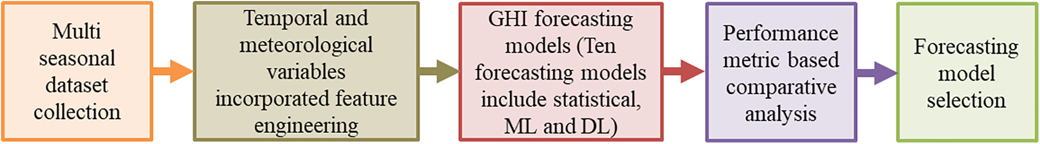
Figure 1: General flowchart of the proposed methodology
1.2 Significant of the Carried Out Performance Analysis
The present research proposes a unique aspect of the engineering framework that optimally integrates meteorological variables with temporal patterns and sky condition indicators. It also provides the first meticulous comparison of ten forecasting approaches (spanning statistical, machine learning, and deep learning paradigms) for global horizontal irradiance prediction across various Indian seasons. The significance of the carried out performance analysis is pointed out as below:
(1) Accomplished Multi seasonal (winter, spring, summer, monsoon, autumn) based on GHI forecasting.
(2) Using temporal patterns and climatic variables in a unique feature engineering framework.
(3) A rigorous benchmarking framework that assesses ten various forecasting models employing identical data. Performed the comparative performance analysis of the 10 forecasting models (ARIMA, Elman network, RBFN, SVM, LSTM, Persistent, BPN, MLP, Random Forest, and XGBoost). The implemented XGboost and random forest-based multi-seasonal GHI forecasting achieved better forecasts than other considered forecasting models.
(4) Performance asses using the India region-based dataset, which comprises the 15 meteorological parameters, including GHI. Therefore, it can be robust about the atmospheric variable-based impact.
(5) MAE, RMSE, and R2 are the performance metrics used to evaluate the all-considered model forecasting ability.
(6) Findings provide beneficial recommendations for energy system operators to select the best forecasting models.
This paper’s remaining sections are organised as follows. The forecasting model design and description are put forward in Section 2. Multi-seasonal-based GHI forecasting results and comparisons are given in the result and discussion Section 3. Lastly, Section 4 provides the conclusion and recommendations.
2 Forecasting Model Design and Description
This section details the dataset, seasons, data preprocessing, splitting and feature engineering, mathematical expressions of the forecasting models, and performance metrics.
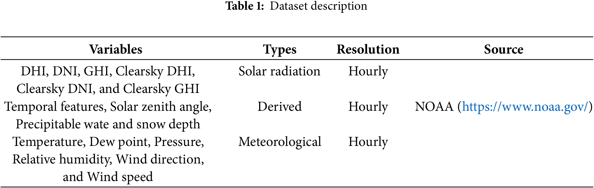
The data set from the region of Pavagada, Karnataka, India, for a period of the year, is gathered from the NOAA (National Oceanic and Atmospheric Administration), which consists of the hourly-based dataset comprising 8760 data samples of each variable likes DHI (Diffuse Horizontal Irradiance), DNI (Direct Normal Irradiance), GHI, Clearsky DHI, Clearsky DNI, Clearsky GHI, Dew Point, Temperature, Pressure, Relative Humidity, Solar Zenith Angle, Precipitable Water, Snow Depth, Wind Direction, and Wind Speed. The data description variables, types, resolution and source are clearly mentioned in Table 1.
Seasons
This paper uses the India region dataset, focusing on the five seasons: winter, spring, summer, monsoon and autumn. India’s seasons are mostly categorised as spring, which continues from February to March. The monsoon season is present from March to May, summer, and June to September. Autumn, which lasts from October to November. December through February is winter.
2.2 Data Preprocessing, Splitting and Feature Engineering
The data preprocessing, data splitting and feature engineering are detailed as follows:
Data preprocessing comprises data missing handling, outlier removal, and z-core normalisation [19].
where,
Data splitting into training and testing. Training uses 70% of the data, and testing uses 30%. Test data are necessary for the model’s performance analysis, which analyses every forecast model’s accuracy. The forecasting model must not be trained using the same dataset as the test. To enhance forecast performance, feature engineering is the procedure of generating more details from the data.
This work used the time features, lag features and meteorological features.
Temporal Features: Two significant cyclical temporal characteristics are extracted such as Hours of day (0–23) to record trends throughout the day and Year of the year (1–365) to record seasonal changes. These are especially crucial for simulating solar radiation, since GHI exhibits substantial daily and seasonal variations.
Lag Features: The GHI time series’ temporal dependencies are better captured by these autoregressive properties.
Selection of Meteorological Features:
First, every collected meteorological feature is accessible and maintains characteristics that are physically related to sun radiation and drop characteristics with no variance. Both actual meteorological features and calculated sun angles are included in the final features. Additionally, selecting features, such as preserving the top fifteen features using mutual information scoring, Multicollinearity control with VIF < 5 and winter concentrates on cloud clues (dew point), whilst the monsoon season includes features connected to precipitation and wind. For time-series data, such as hourly GHI, lag characteristics are used to represent historical values. To determine the periodicity, take the time stamps and extract the hour, day, month, and weekdays. The DHI, DNI, GHI, Clearsky DHI, Clearsky DNI, Clearsky GHI, Dew Point, Temperature, Pressure, Relative Humidity, Solar Zenith Angle, Precipitable Water, Snow Depth, Wind Direction, and Wind Speed meteorological parameters. GHI may frequently be forecasted based on these features and characteristics.
2.3 Mathematical Expressions of the Forecasting Models
The considered all forecasting models such as ARIMA (Autoregressive Integrated Moving Average), Elaman NN (Elman Neural Network), RBFN (Radial Basis Function Neural Network), SVM (Support Vector Machine), LSTM (Long Short-Term Memory), Persistent, BPN (Back Propagation Neural Network), MLP (Multilayer Perceptron Neural Network), RF (Random Forest), and XGBoost (eXtreme Gradient Boosting) simplified description, mathematical expressions are as follows:
AutoRegressive Integrated Moving Average (ARIMA): ARIMA is a statistics model employed in forecasting and time series analysis [20]. When confronted with a non-stationary time series, it combines moving average and autoregressive constituents with an integration step.
where,
Stationarity handling: The Dickey-Fuller test demonstrated stationarity non-stationarity (p = 1) following first-order differencing using autocorrelation plots directing AR(1) and MA(1) term choice [21].
Elman Neural Network (ENN): To analyse sequential input, the Elman Neural Network, a kind of feedback neural network, retains information about prior time steps in a context layer [22].
where,
Radial Basis Function Network (RBFN): RBFN is a feedforward network in which the network’s second layer is weighted, and the number of inputs is equal to the size of the hidden layer, which comprises nonlinear radial basis functions [23]. The output neurons are simple summing junctions.
where,
Support Vector Machine (SVM): To classify data points, even though they are not generally linearly separable, SVM maps the data to a high-dimensional feature space [24]. Once a hyperplane is identified between the groups, the data is altered.
where,
Long Short-Term Memory (LSTM): In an effort to address the vanishing gradient issue that conventional RNNs commonly encounter, long short-term memory (LSTM), a kind of recurrent neural network (RNN), employs “gates” that retrieve both long-term and short-term memory [25].
where,
Persistent: Forecasts today using the GHI value from the previous day are the fundamental concept of the Persistent forecast. Difficult to identify trends beyond daily tenacity.
Backpropagation Network (BPN): The Deepest-Descent method is the foundation of the learning process used by the BPNN.
where,
Multilayer Perceptron (MLP): A feedforward neural network with completely linked neurons having nonlinear activation functions arranged in layers is referred to as a multilayer perceptron (MLP) [26].
where,
Random Forest (RF): An ensemble learning technique for regression and other problems built on many decision trees during training and then averages the results [27].
where,
XGBoost (eXtreme Gradient Boosting): To enhance the model’s effectiveness, XGBoost employs decision trees as its foundational learners and combines each of them sequentially [28]. The computational efficiency, smooth handling of missing values, and efficient processing are the significant features of the XGBoost.
where,
The hyperparameters for each model were chosen based on the domain expertise and trial and error. Table 2 presents a hyperparameter used for every designed forecasting model and, with the carefully selected hyperparameters to avoid overfitting, maintained manageable training periods while offering enough capacity to learn intricate patterns. Table 2, based on set values hyperparameters, provides the optimal trade-off between training time and forecasting performance without overfitting and captured temporal relationships. The performance analysis workflow is shown in Fig. 2.
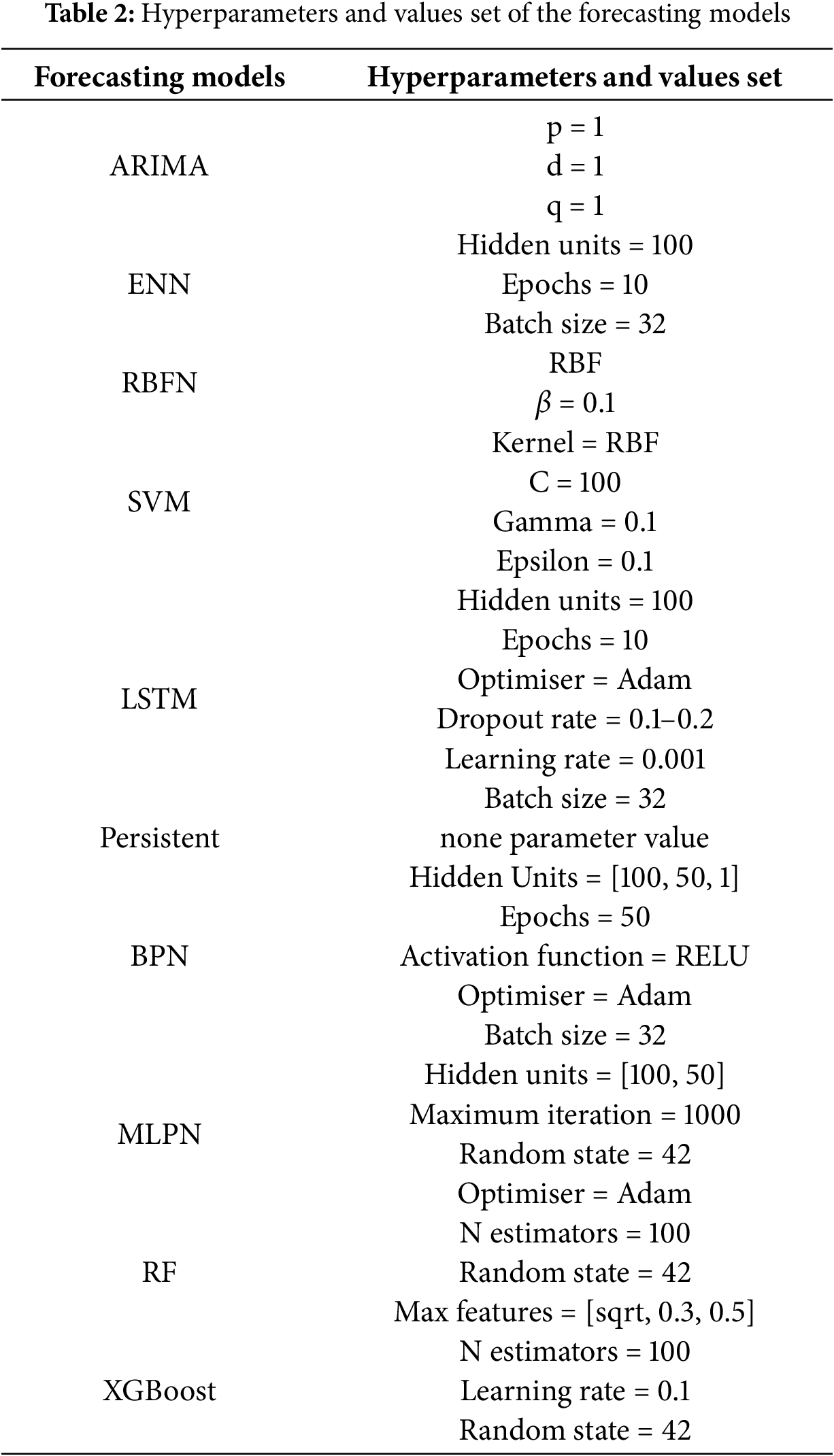
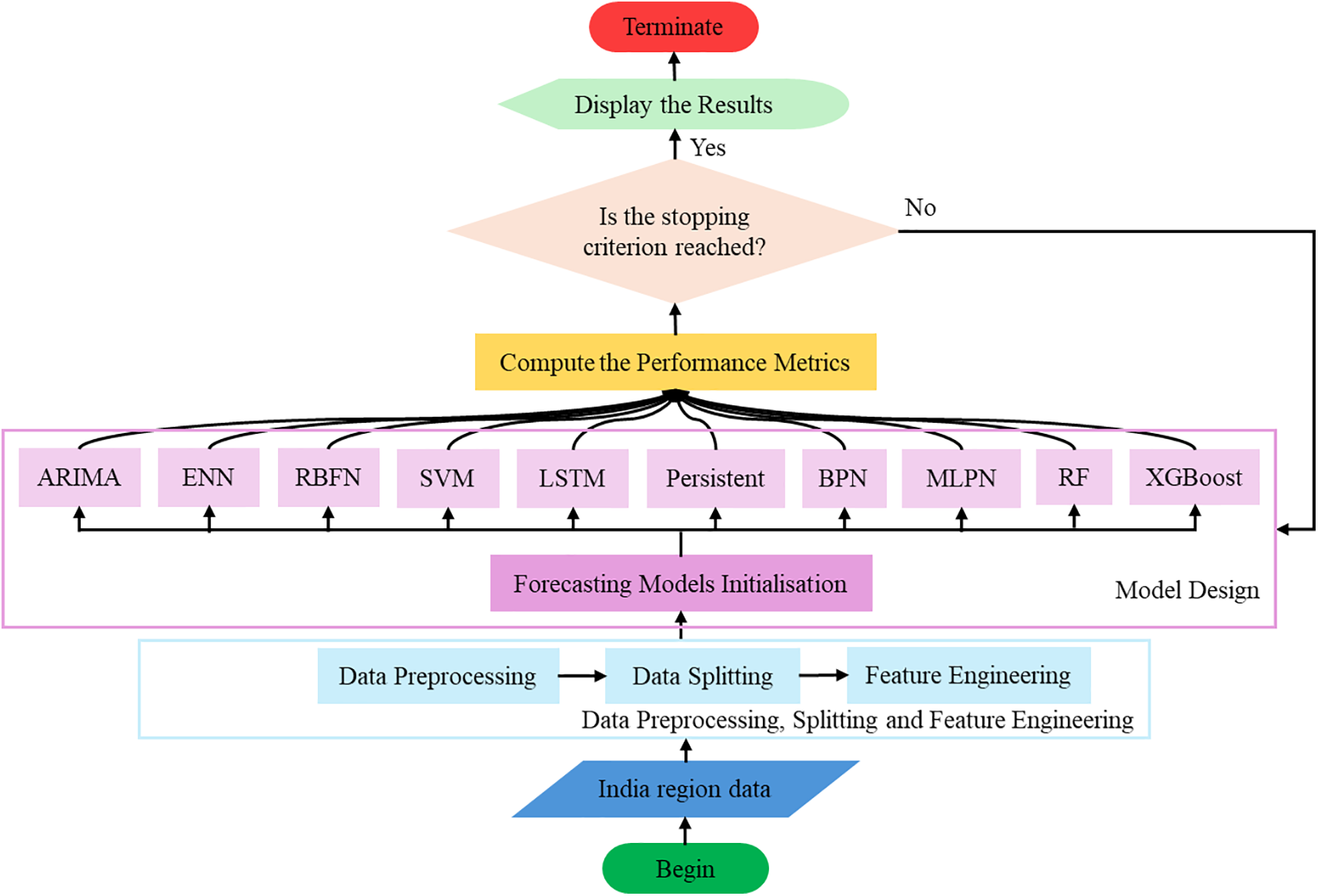
Figure 2: Flowchart of the proposed performance analysis multi-seasonal global horizontal irradiance forecasting
The designed all-seasons-based GHI forecasting model’s performances are evaluated using performance metrics such as Mean Absolute Error (MAE) [29], Root Mean Squared Error (RMSE) [30], and R-squared (R2) [14].
MAE (Mean Absolute Error)
The average of the actual variations between the forecast values is referred to as MAE.
RMSE (Root Mean Squared Error)
The square root of the mean of the squared variations between the actual and forecast values is referred to as RMSE.
R-squared (R2)
The coefficient of multiple correlation’s square is referred to as R2, which commonly lies between 0 and 1.
where,
An AMD Ryzen™ 7 PRO 7840U CPU operating at 3301 MHz with 16 GB of RAM, a Lenovo Thinkpad T16 Gen 2, a Spyder IDE version 5.5.1 (Conda), and Python 3.12.7 64-bit were used for the experiment to simulate the all the considered forecasting models using the India region dataset.
Multi-Seasonal Global Horizontal Irradiance Forecasting
Each model’s based multi-seasonal forecasting comparison of the actual vs. forecasts is shown in Figs. 3–7 are testing datasets based on achieved results. It is evident that XGboost and RF are closely matched with the actual GHI, whereas XGBoost has the lowest and ARIMA, Elman, RBFN, and LSTM yield the worst matched with the actual GHI. Between the RF and XGboost-based models, there is minimal variation. The XGboost and RF models compete with each other in the deterministic forecast of India region’s actual data sets compared to other forecasting models used for the comparative performance analysis.
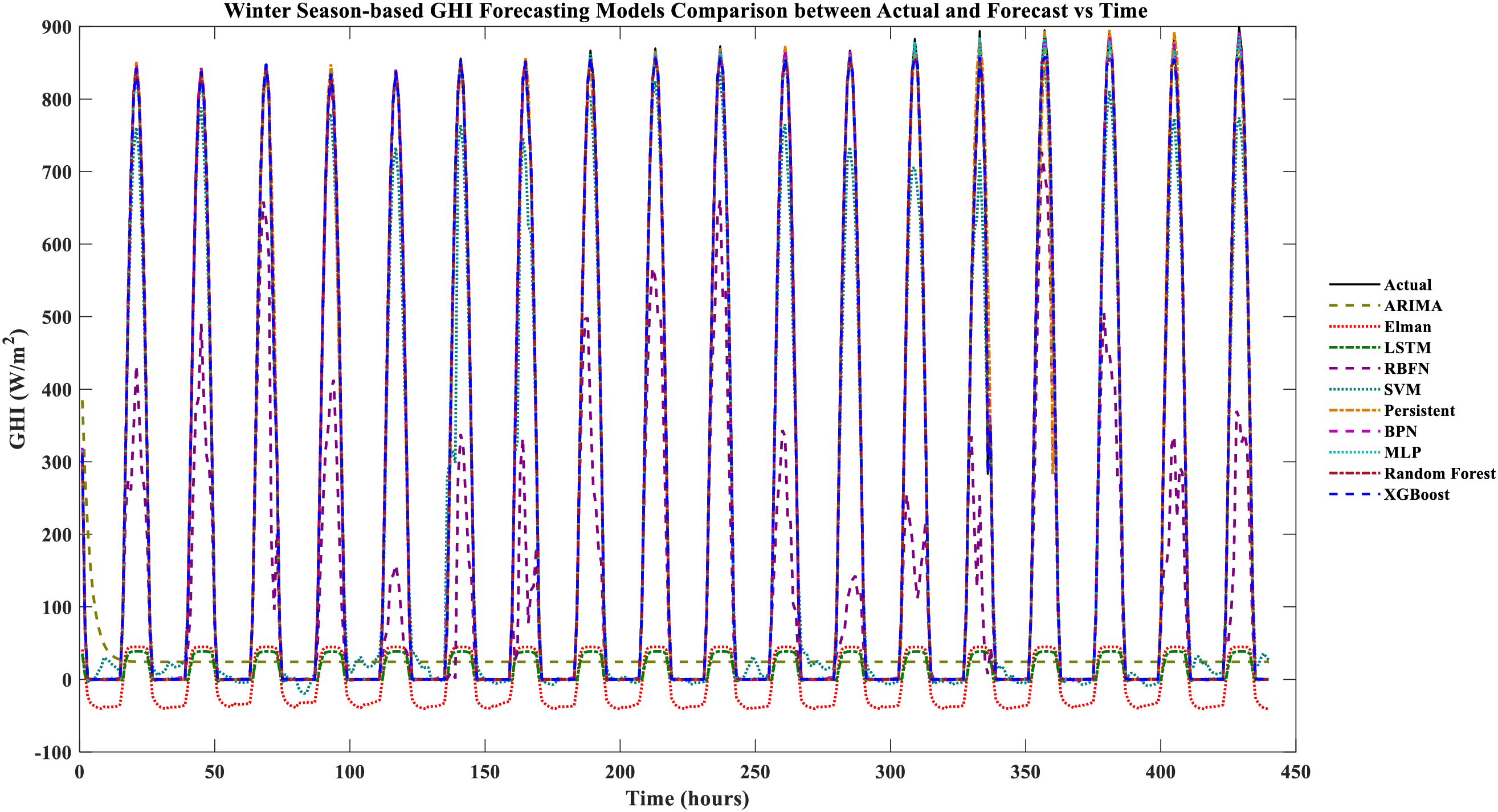
Figure 3: Winter season-based GHI forecasting models comparison between actual and forecast vs. time
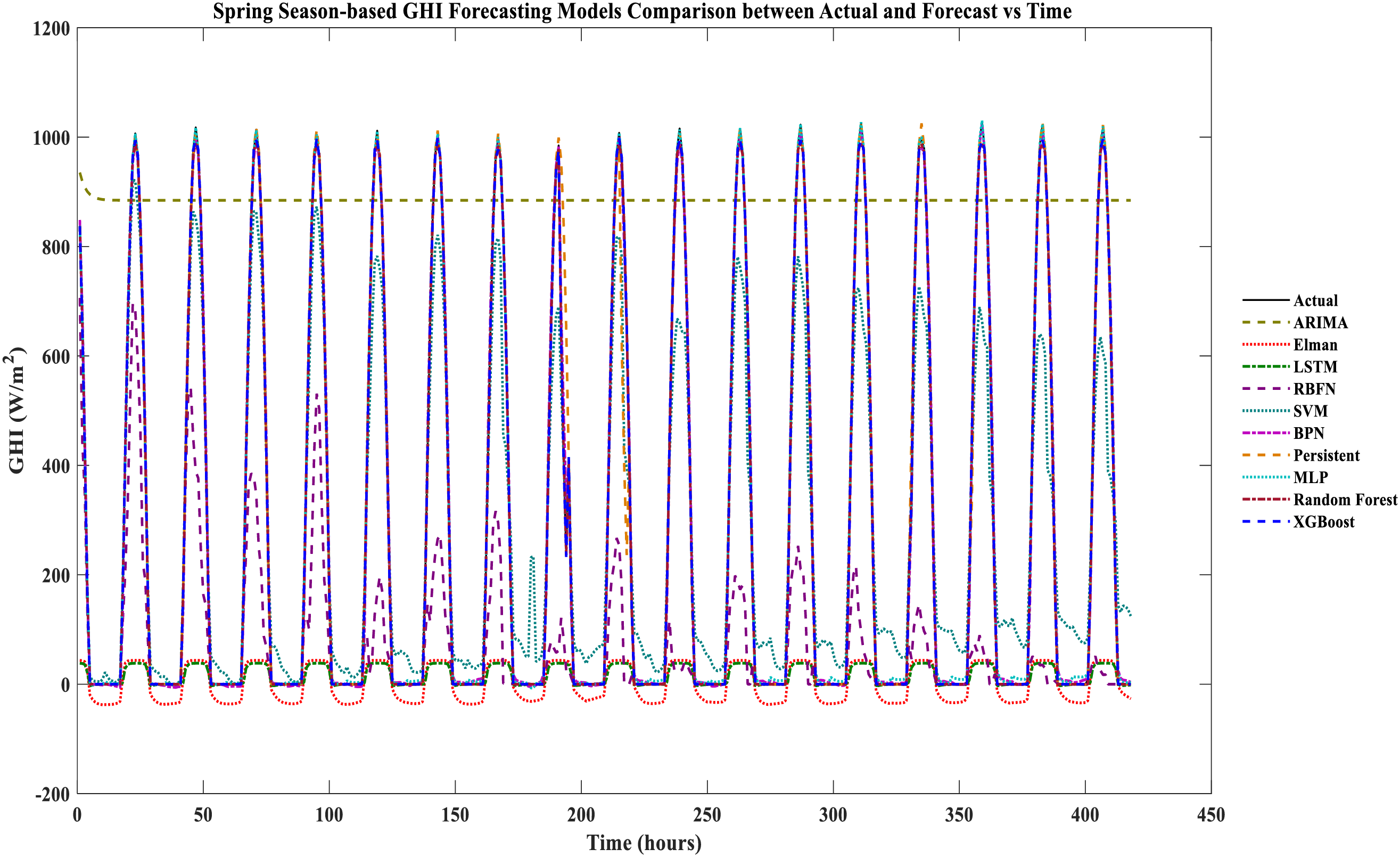
Figure 4: Spring season-based GHI forecasting models comparison between actual and forecast vs. time
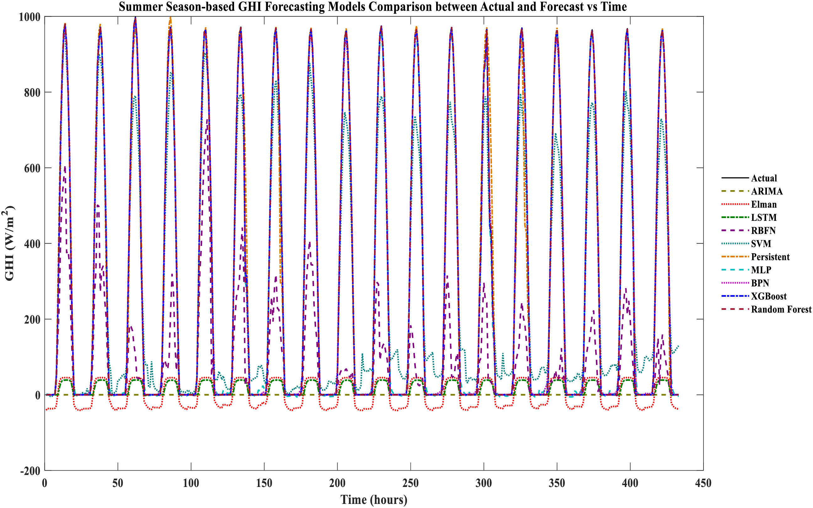
Figure 5: Summer season-based GHI forecasting models comparison between actual and forecast vs. time
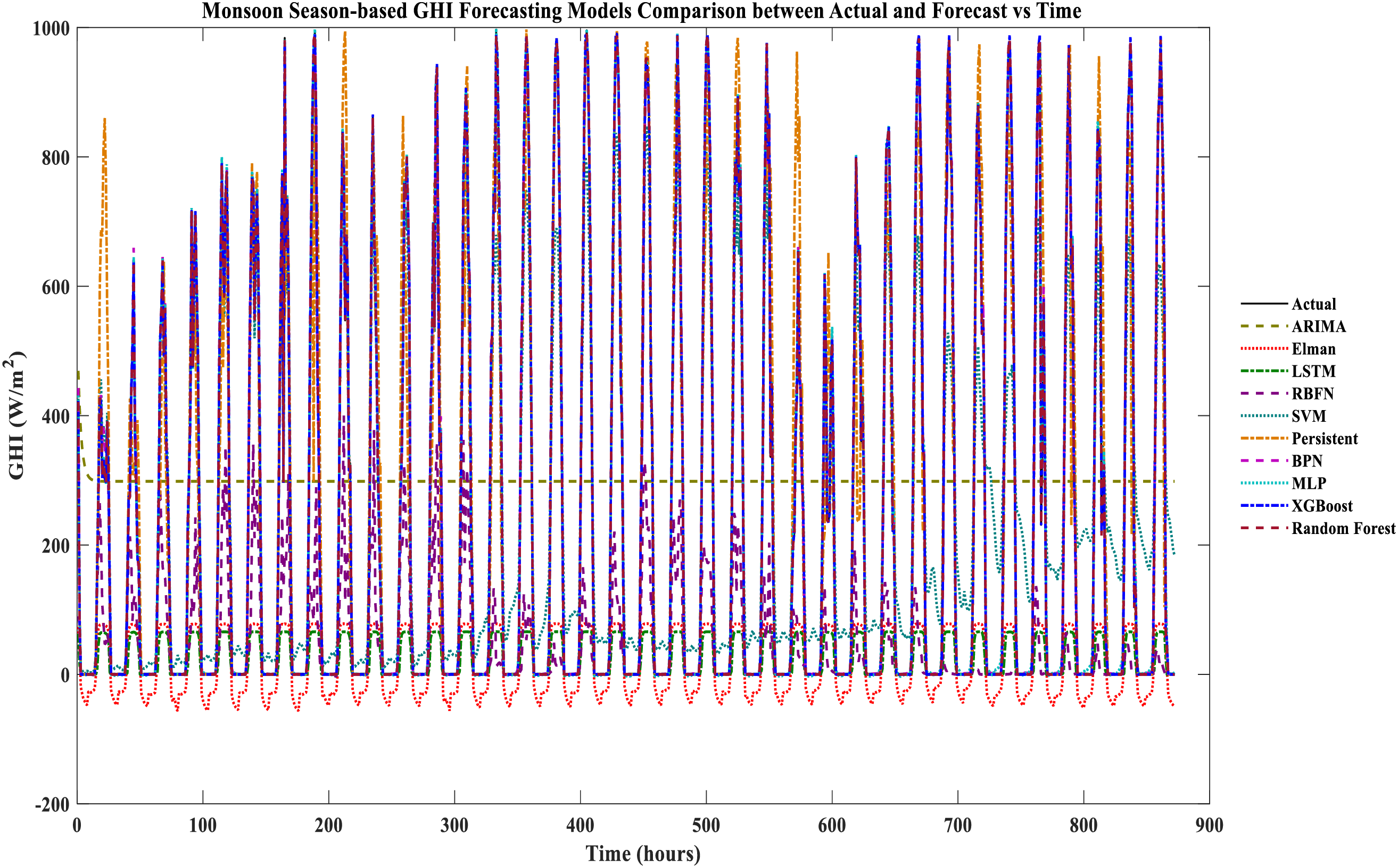
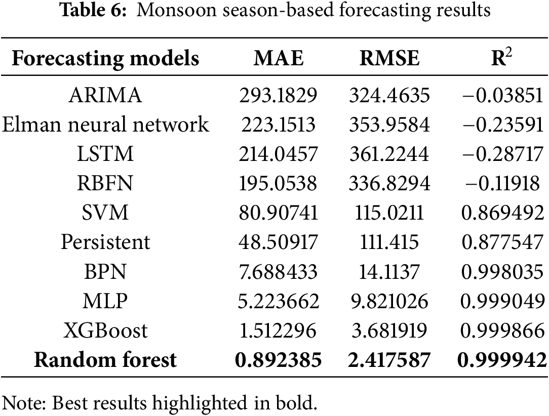
Figure 6: Monsoon season-based GHI forecasting models comparison between actual and forecast vs. time
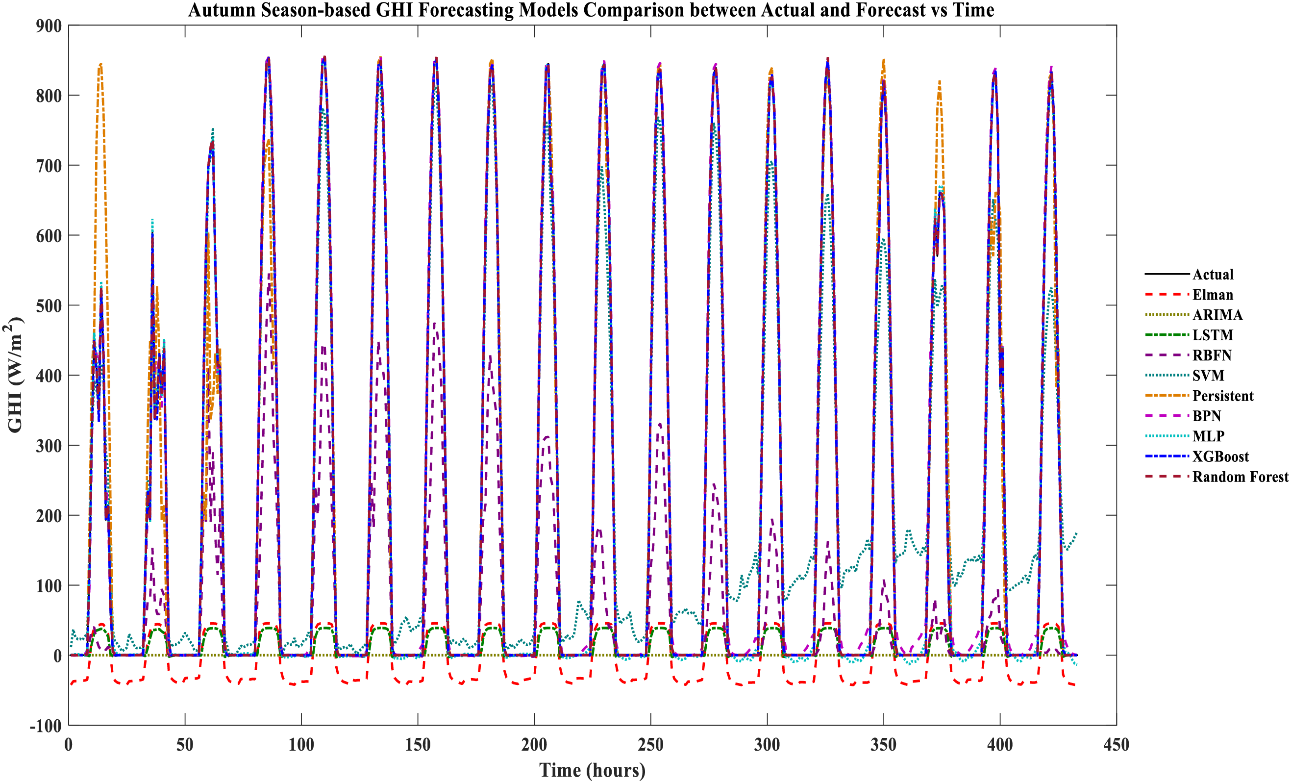
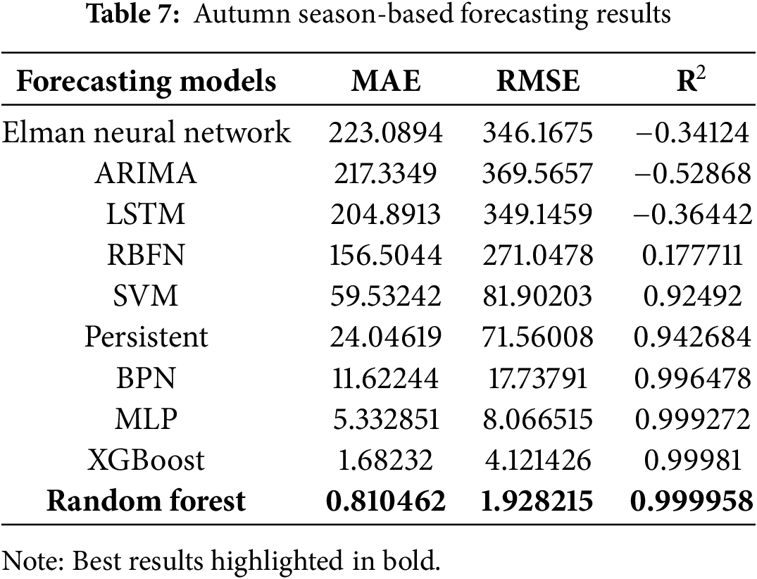
Figure 7: Autumn season-based GHI forecasting models comparison between actual and forecast vs. time
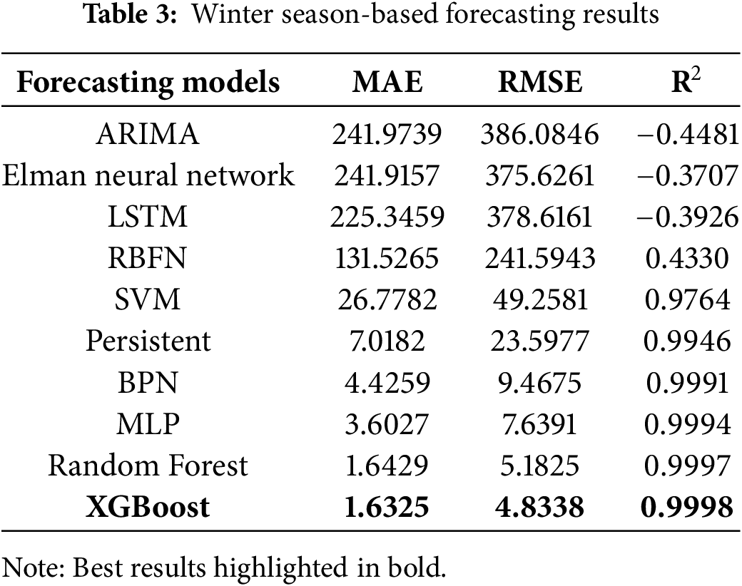
The forecasting models were used to build and evaluate the forecast for multiple seasons using the India region dataset, resulting in performance metrics for the various seasons listed in Tables 3–7. It can be seen in Table 3. Winter season-based forecasting results performance metrics. XGBoost is the best forecasting model among the other models that yield the least performance metrics, such as MAE: 1.6325, RMSE: 4.8338, and R2: 0.9998. RF model yields the competing performance metrics, while MLP, BPN, persistent, and SVM-based models yield moderate forecasting performance. ARIMA, Elman, LSTM, and RBFN-based models yield the worst performance metrics.
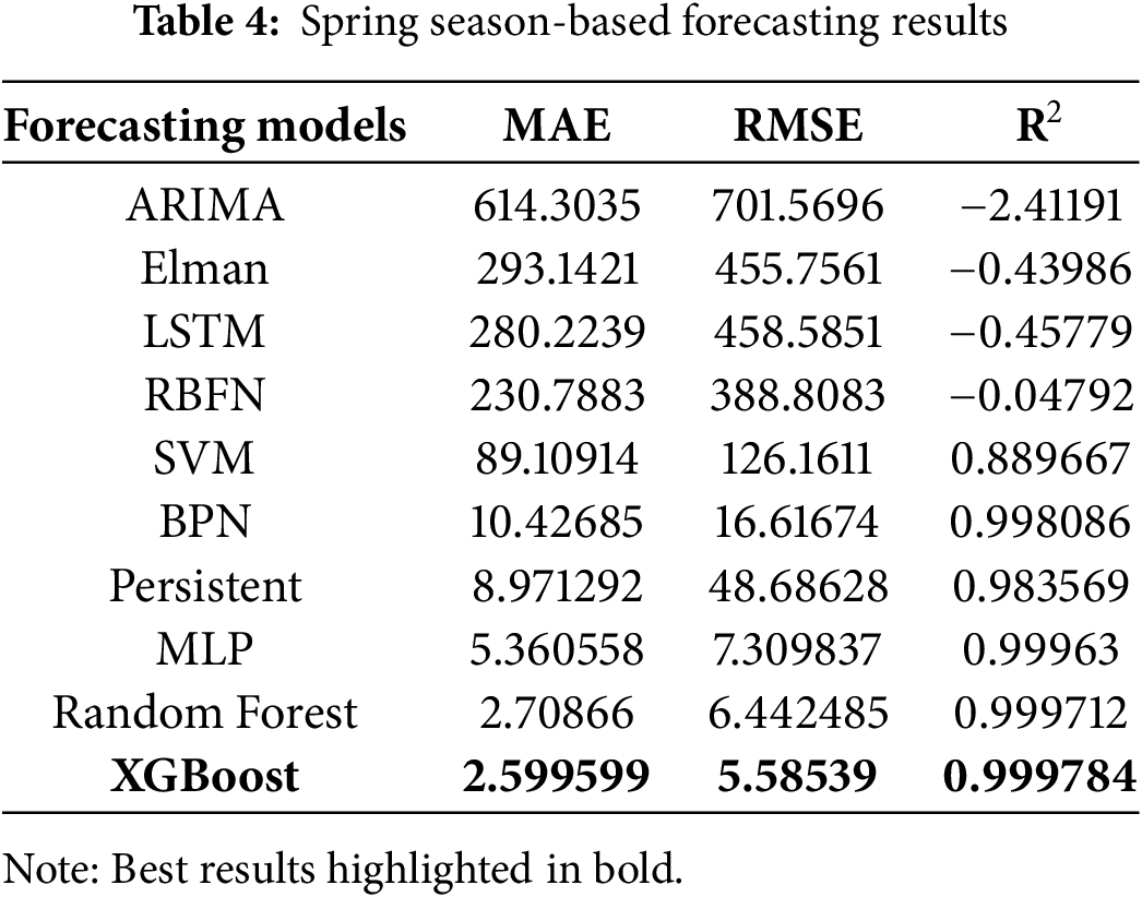
From Table 4, spring season-based forecasting results performance metrics. ARIMA, Elman, LSTM, and RBFN yield the worst performance metrics. MLP, persistent, BPN, and SVM-based models yield moderate forecasting performance. RF model yields the competing performance metrics, and XGBoost is the best forecasting model among the other models that yield the least performance metrics, such as MAE: 2.599599, RMSE: 5.58539, and R2: 0.999784.
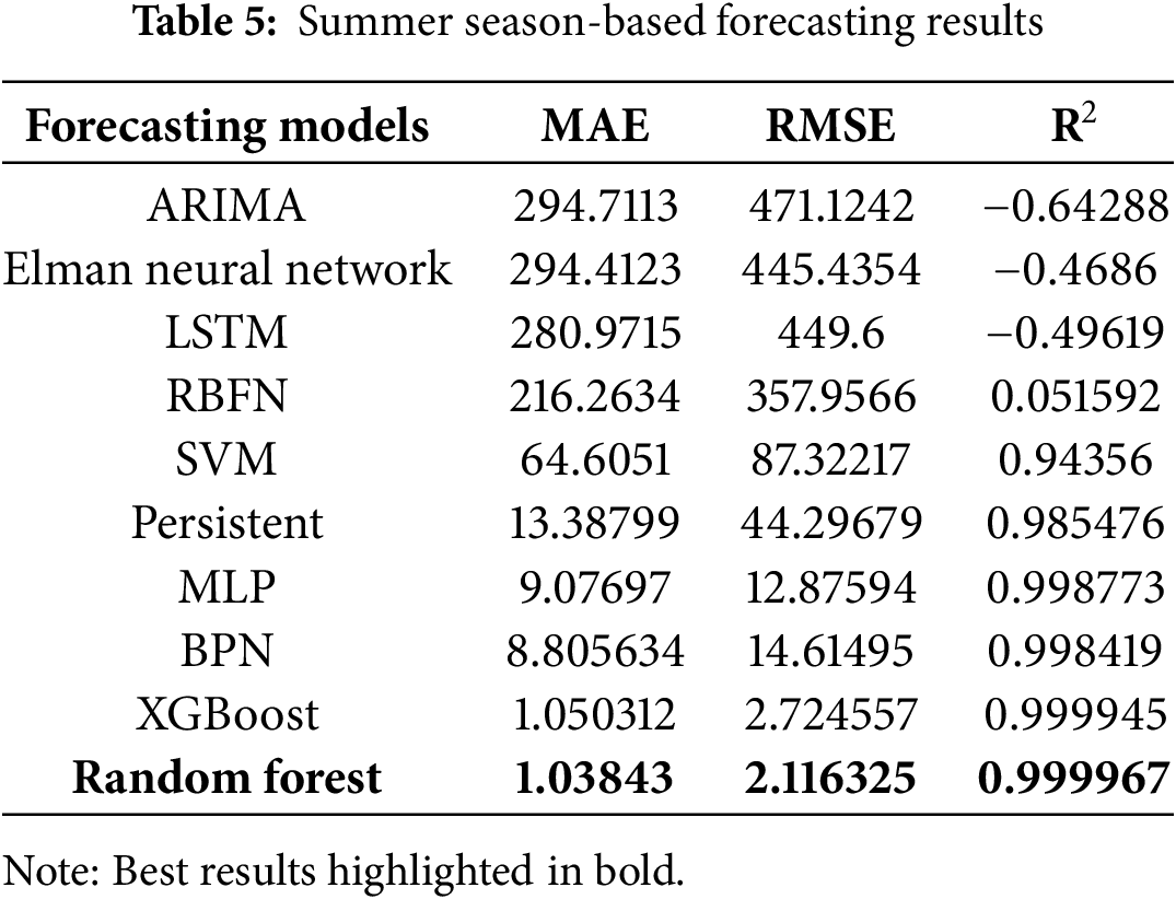
It can be noticed from Table 5, summer season-based forecasting results performance metrics. RF is the best forecasting model among the other models that yield the least performance metrics, such as MAE: 1.03843, RMSE: 2.116325, and R2: 0.999967. XGBoost model yields the competing performance metrics, and BPN, MLP, persistent, and SVM-based models yield moderate forecasting performance. ARIMA, Elman, LSTM, and RBFN-based models yield the worst performance metrics inferred from Table 6. Monsoon season-based forecasting results performance metrics. ARIMA, Elman, LSTM, and RBFN yield the worst performance metrics. MLP, BPN, persistent, and SVM-based models yield moderate forecasting performance. XGBoost model yields the competing performance metrics, and RF is the best forecasting model among the other models yielding the least performance metrics, such as MAE: 0.892385, RMSE: 2.417587, and R2: 0.999942.
It can be noticed in Table 7, autumn season-based forecasting results performance metrics. RF is the best forecasting model among the other models with the least performance metrics, such as MAE: 0.810462, RMSE: 1.928215, and R2: 0.999958. XGBoost model yields the competing performance metrics.
MLP, BPN, persistent and SVM-based models are yielding moderate forecasting performance. Elman, ARIMA, LSTM, and RBFN-based models yield the worst performance metrics. For a better visualisation of the result, performance metrics, Fig. 8a–e are presented. As a result, RF and XGBoost models are more suited to forecast multi-seasonal-based GHI forecasting. Autumn season-based results are highly likely to match the actual GHI results, the lowest performance metric clearly understood in Fig. 8 and Tables 3–7.
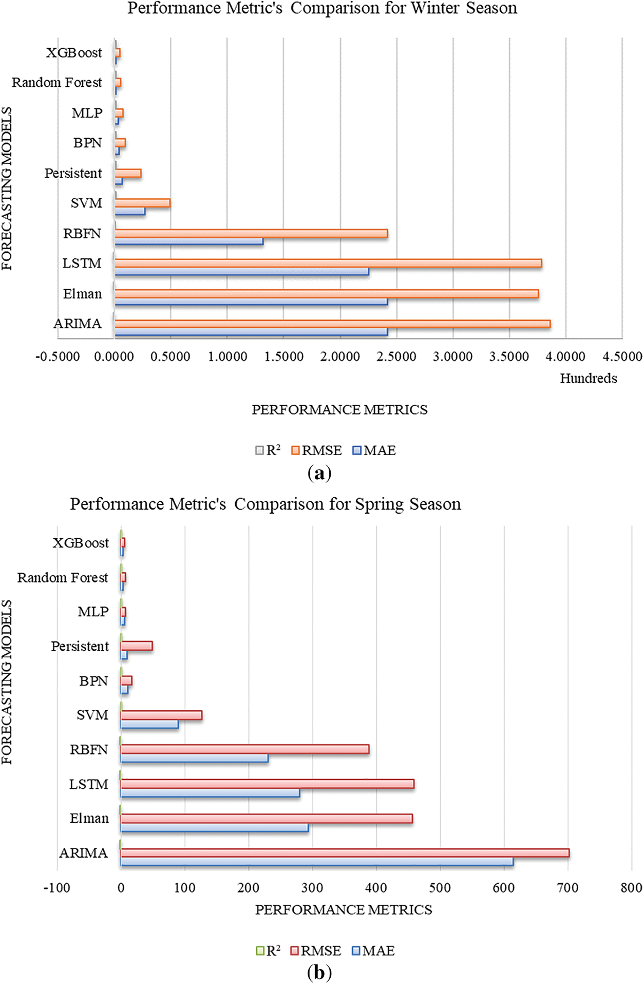
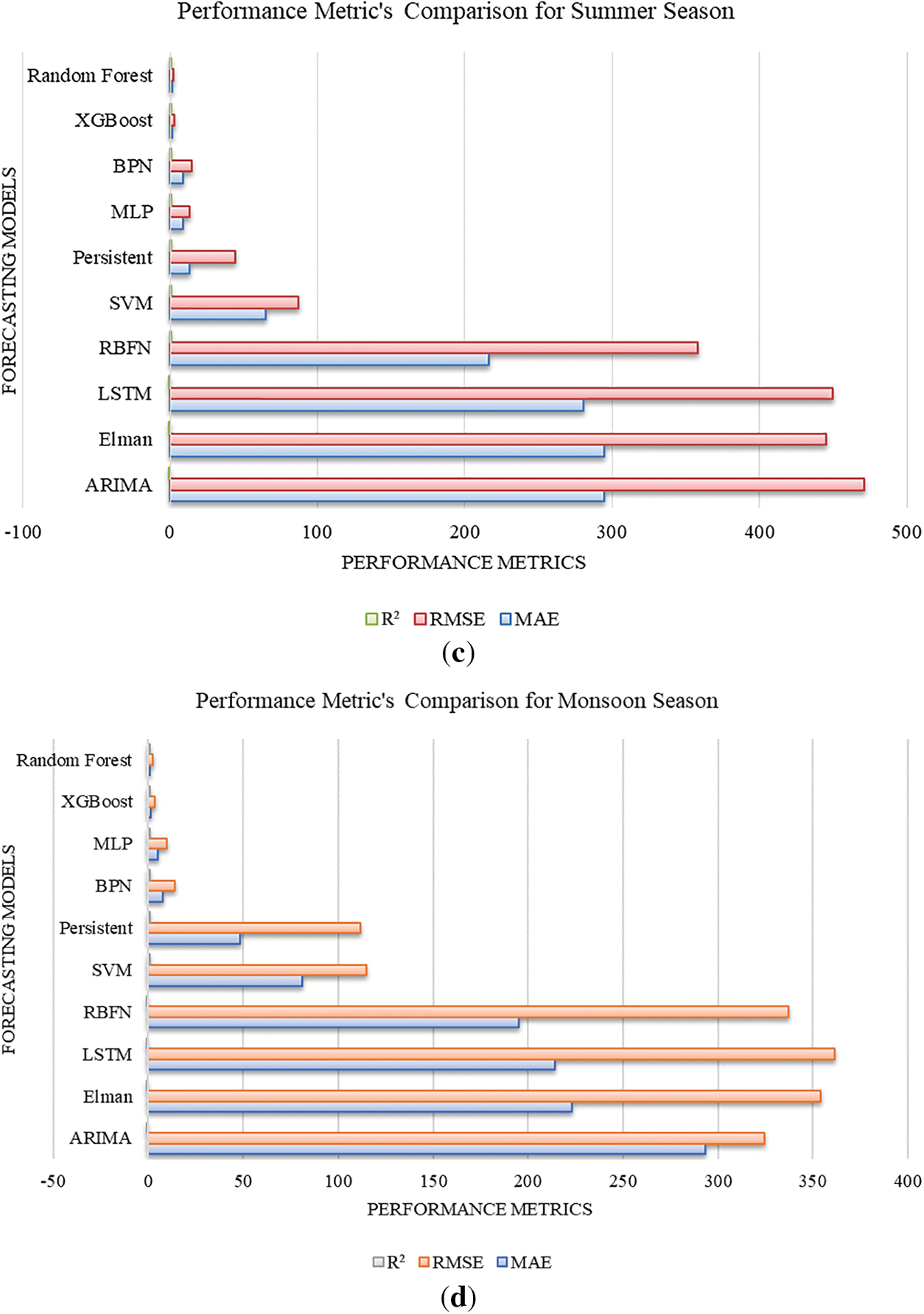
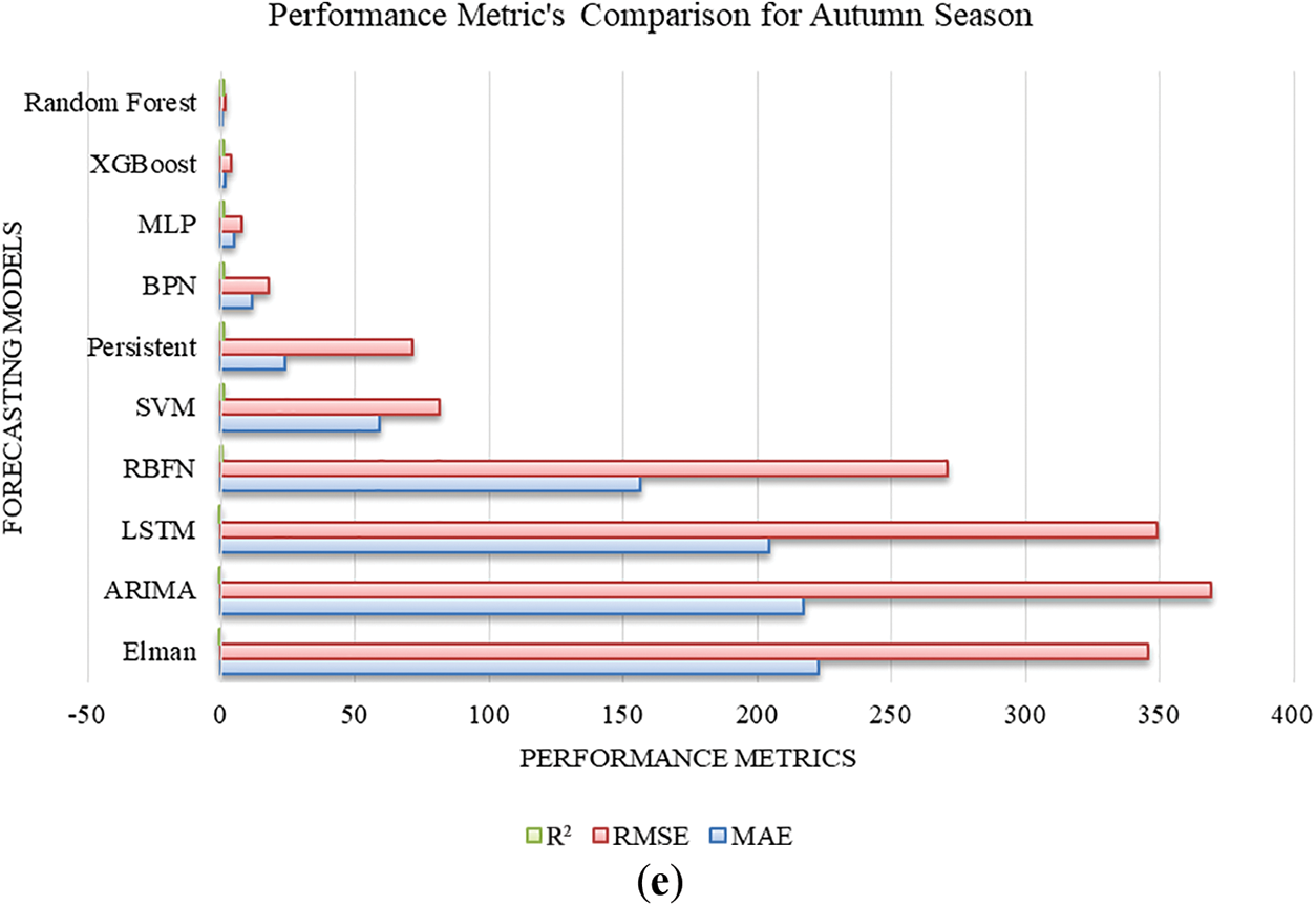
Figure 8: Performance Metrics comparison for (a) Winter season, (b) Spring season, (c) Summer season, (d) Monsoon season, (e) Autumn season
Despite estimating put-off GHI values, feature importance research revealed that the Solar Radiation, Derived and Meteorological type features and temporal features were consistently among the best forecasters for every season. This physical consistency raises the model’s generalizability confidence level. The findings show that the effectiveness of the forecasting model varies significantly with the seasons. This paper compares performance analysis, which can improve solar power system efficiency and allow for more efficient integration of the solar input into the electrical grid using the suggested forecasting models. The significant findings of the carried out performance analysis are rigorously assessing 10 forecasting models’ performance in the India region throughout various seasons and showing notable seasonal variations regarding the performance of the models. Temporal, lag and meteorological feature importance illustrate seasonal variations. Research has demonstrated that the optimal trade-off between accuracy and computational burden is frequently offered by simpler models (XGBoost) and RF. Additionally, it provides explicit guidelines on forecasting model selection based on various seasons, making it a helpful reference for GHI forecasting than the existing research available in the literature.
Considering the severe difficulties that Mother Earth faces from climate change and global warming. A near-real-time prediction model that can aid in more efficient use of solar power is necessary due to the intermittent nature of solar energy, a reason that the share of solar energy worldwide is steadily rising with the use of solar energy systems in distributed systems. GHI is unlikely to be accurately predicted because of the influence of swift changes in weather conditions and meteorological parameters. Solar energy is the growing energy sector worldwide, and concern is required for the effective integration of solar energy with the astute multi-seasonal forecasting of GHI. This research work was carried out to design a solar GHI forecasting system using various models such as ARIMA, Elman, LSTM, RBFN, SVM, persistent, BPN MLP, RF, and XGBoost analysis of various India seasons-based GHI forecasting. In comparison to the other forecasting models, the RF and XGBoost are the best and most competitive models that provide the most accurate forecasts throughout all seasons, according to the performance analysis. Forecasting using winter with an R2 of 0.9998, an RMSE of 4.8338, and an MAE of 1.6325, XGBoost is the best forecasting model. Through an R2 of 0.999784, RMSE of 5.58539, and MAE of 2.599599, XGBoost is the best forecasting model based on spring. With an R2 of 0.999967, RMSE of 2.116325, and MAE of 1.03843, the RF is the best forecasting model based on summer. With R2: 0.999942, RMSE: 2.417587, and MAE: 0.892385, RF is Monsoon’s best forecasting model. Through an R2 of 0.999958, RMSE of 1.928215, and MAE of 0.810462, RF is the best forecasting model for autumn. The primary benefit of the performance analysis using GHI forecast aid in smart grid infrastructure development is that it lowers the likelihood of power management issues, flexibility reserve needs, and energy imbalance markets. The performance analysis reveals that the RF and XGBoost forecasting models can effectively achieve high-precision forecasting in smart grids under various seasonal circumstances with the least performance metrics than the other forecasting models considered for comparison. In the future, the paper can be extended to focus on the issues related to the forecast model (XGBoost and RF), such as overfitting and proper selection of the hyperparameter. Hence, the optimisation algorithm optimises and validates the forecasting model design with different region datasets, which confirms the generalisation ability.
Acknowledgement: The author wishes to thank the NOAA for the dataset.
Funding Statement: The author received no specific funding for this study.
Availability of Data and Materials: The data analysed in this study was obtained from the National Oceanic and Atmospheric Administration, and restrictions apply to access the datasets. Requests to access these datasets should be directed to the National Oceanic and Atmospheric Administration official website https://www.noaa.gov/.
Ethics Approval: Not applicable.
Conflicts of Interest: The author declares no conflicts of interest to report regarding the present study.
Glossary
| ARIMA | Autoregressive Integrated Moving Average |
| Elman NN | Elman Neural Network |
| RBFN | Radial Basis Function Neural Network |
| SVM | Support Vector Machine |
| LSTM | Long Short-Term Memory |
| BPN | Back Propagation Neural Network |
| MLP | Multilayer Perceptron Neural Network |
| RF | Random Forest |
| XGBoost | eXtreme Gradient Boosting |
| GHI | Global Horizontal Irradiance |
| MAE | Mean Absolute Error |
| RMSE | Root Mean Squared Error |
| R2 | R-squared |
| DHI | Diffuse Horizontal Irradiance |
| DNI | Direct Normal Irradiance |
| SVR | Support Vector Regression |
| GRU | Gated Recurrent Unit neural network |
| GFF | Generalised FeedForward networks |
| SOFM | Self-Organizing Feature Maps |
References
1. Madhiarasan M, Louzazni M. Combined long short-term memory network-based short-term prediction of solar irradiance. Int J Photoenergy. 2022;2022(1):1004051. doi:10.1155/2022/1004051. [Google Scholar] [CrossRef]
2. Solar overview. [cited 2025 Jun 24]. Available from: https://mnre.gov.in/en/solar-overview. [Google Scholar]
3. State wise RE installed capacity as on 31.05.2025. [cited 2025 Jun 23]. Available from: https://cdnbbsr.s3waas.gov.in/s3716e1b8c6cd17b771da77391355749f3/uploads/2025/06/202506131034278891.pdf. [Accessed 26 Jun 2025]. [Google Scholar]
4. Gyeltshen S, Hayashi K, Tao L, Dem P. Statistical evaluation of a diversified surface solar irradiation data repository and forecasting using a recurrent neural network-hybrid model: a case study in Bhutan. Renew Energy. 2025;245(7):122706. doi:10.1016/j.renene.2025.122706. [Google Scholar] [CrossRef]
5. Madhiarasan M, Deepa SN. Deep neural network using new training strategy based forecasting method for wind speed and solar irradiance forecast. Mid-East J Sci Res. 2016;24(12):3730–47. [Google Scholar]
6. Kazem HA, Yousif JH. Comparison of prediction methods of photovoltaic power system production using a measured dataset. Energy Convers Manag. 2017;148(20):1070–81. doi:10.1016/j.enconman.2017.06.058. [Google Scholar] [CrossRef]
7. Srivastava S, Lessmann S. A comparative study of LSTM neural networks in forecasting day-ahead global horizontal irradiance with satellite data. Sol Energy. 2018;162(3):232–47. doi:10.1016/j.solener.2018.01.005. [Google Scholar] [CrossRef]
8. Li X, Ma L, Chen P, Xu H, Xing Q, Yan J, et al. Probabilistic solar irradiance forecasting based on XGBoost. Energy Rep. 2022;8(1):1087–95. doi:10.1016/j.egyr.2022.02.251. [Google Scholar] [CrossRef]
9. Sravankumar J, Josh FT, Stonier AA, Peter G, Jayaraj J, Jaganathan S, et al. Random forest machine learning algorithm based seasonal multi-step ahead short-term solar photovoltaic power output forecasting. IET Renew Power Gener. 2025;19(1):e12921. doi:10.1049/rpg2.12921. [Google Scholar] [CrossRef]
10. Chodakowska E, Nazarko J, Nazarko Ł, Rabayah HS, Abendeh RM, Alawneh R. ARIMA models in solar radiation forecasting in different geographic locations. Energies. 2023;16(13):5029. doi:10.3390/en16135029. [Google Scholar] [CrossRef]
11. Sedai A, Dhakal R, Gautam S, Dhamala A, Bilbao A, Wang Q, et al. Performance analysis of statistical, machine learning and deep learning models in long-term forecasting of solar power production. Forecasting. 2023;5(1):256–84. doi:10.3390/forecast5010014. [Google Scholar] [CrossRef]
12. Gupta R, Yadav AK, Jha SK, Pathak PK. Predicting global horizontal irradiance of north central region of India via machine learning regressor algorithms. Eng Appl Artif Intell. 2024;133(3):108426. doi:10.1016/j.engappai.2024.108426. [Google Scholar] [CrossRef]
13. Tandon A, Awasthi A, Pattnayak KC, Tandon A, Choudhury T, Kotecha K. Machine learning-driven solar irradiance prediction: advancing renewable energy in Rajasthan. Discov Appl Sci. 2025;7(2):107. doi:10.1007/s42452-025-06490-8. [Google Scholar] [CrossRef]
14. Madhiarasan M. Bayesian optimisation algorithm based optimised deep bidirectional long short term memory for global horizontal irradiance prediction in long-term horizon. Front Energy Res. 2025;13:1499751. doi:10.3389/fenrg.2025.1499751. [Google Scholar] [CrossRef]
15. Gupta R, Yadav AK, Jha SK, Pathak PK. Composition of feature selection techniques for improving the global horizontal irradiance estimation via machine learning models. Therm Sci Eng Prog. 2024;48(2):102394. doi:10.1016/j.tsep.2024.102394. [Google Scholar] [CrossRef]
16. Gupta R, Yadav AK, Jha SK, Pathak PK. A robust regressor model for estimating solar radiation using an ensemble stacking approach based on machine learning. Int J Green Energy. 2024;21(8):1853–73. doi:10.1080/15435075.2023.2276152. [Google Scholar] [CrossRef]
17. El Ouiqary A, Kheddioui EM, Smiej MF. Evaluation of the Global Horizontal Irradiation (GHI) on the ground from the images of the second generation european meteorological satellites MSG. J Comput Commun. 2023;11(1):1. doi:10.4236/jcc.2023.111001. [Google Scholar] [CrossRef]
18. Vanlalchhuanawmi C, Deb S, Islam MM, Ustun TS. Solar radiation prediction: a multi-model machine learning and deep learning approach. AIP Adv. 2025;15(5):978. doi:10.1063/5.0237246. [Google Scholar] [CrossRef]
19. Tawari A, Trivedi MM. Speech emotion analysis: exploring the role of context. IEEE Trans Multimed. 2010;12(6):502–9. doi:10.1109/tmm.2010.2058095. [Google Scholar] [CrossRef]
20. Box GE, Jenkins GM, Reinsel GC, Ljung GM. Time series analysis: forecasting and control. 5th ed. Hoboken, NJ, USA: John Wiley & Sons; 2015. [Google Scholar]
21. Dickey DA, Fuller WA. Distribution of the estimators for autoregressive time series with a unit root. J Am Stat Assoc. 1979;74(366a):427–31. doi:10.1080/01621459.1979.10482531. [Google Scholar] [CrossRef]
22. Elman JL. Finding structure in time. Cogn Sci. 1990;14(2):179–211. [Google Scholar]
23. Lowe D, Broomhead D. Multivariable functional interpolation and adaptive networks. Complex Syst. 1988;2(3):321–55. [Google Scholar]
24. Cortes C, Vapnik V. Support-vector networks. Mach Learn. 1995;20(3):273–97. doi:10.1007/bf00994018. [Google Scholar] [CrossRef]
25. Hochreiter S, Schmidhuber J. Long short-term memory. Neural Comput. 1997;9(8):1735–80. doi:10.1162/neco.1997.9.8.1735. [Google Scholar] [PubMed] [CrossRef]
26. Rosenblatt F. The perceptron: a probabilistic model for information storage and organisation in the brain. Psychol Rev. 1958;65(6):386. [Google Scholar] [PubMed]
27. Breiman L. Random forests. Mach Learn. 2001;45:5–32. [Google Scholar]
28. Chen T, He T, Benesty M, Khotilovich V, Tang Y, Cho H, et al. XGBoost: extreme gradient boosting. R Package Version 04-2; 2015 [cited 2025 June 25]. Available from: https://cran.r-project.org/web/packages/xgboost/xgboost.pdf. [Google Scholar]
29. Willmott CJ, Matsuura K. Advantages of the mean absolute error (MAE) over the root mean square error (RMSE) in assessing average model performance. Clim Res. 2005;30(1):79–82. doi:10.3354/cr030079. [Google Scholar] [CrossRef]
30. Madhiarasan M, Louzazni M. Analysis of artificial neural network: architecture, types, and forecasting applications. J Electr Comput Eng. 2022;2022(1):5416722. doi:10.1155/2022/5416722. [Google Scholar] [CrossRef]
Cite This Article
 Copyright © 2025 The Author(s). Published by Tech Science Press.
This work is licensed under a Creative Commons Attribution 4.0 International License , which permits unrestricted use, distribution, and reproduction in any medium, provided the original work is properly cited.
 Downloads
 Citation Tools