1 Introduction
As summarized in previous studies, there are two contradictory views on the dynamic response of aqueducts under lateral seismic excitation [1]: (1) When the natural frequency of the water is close to that of the aqueduct, the water can absorb part of the structural vibration energy and reduce the vibration amplitude of the aqueduct to some extent (e.g., Refs. [2,3,4]). (2) Due to the fluid-structure interaction (FSI) between the water and the aqueduct, the presence of water can increase the dynamic response of the aqueduct (e.g., Refs. [5,6]). Similar to the research on the FSI dynamic response of aqueducts, current studies on liquid sloshing mainly focus on the improvement and comparison of numerical simulation methods (e.g., Refs. [7,8,9]), sloshing characteristics under complex conditions (e.g., Refs. [10,11,12]), the influence of viscosity (e.g., Ref. [13]), and some engineering applications (e.g., Refs. [14,15]). And in the field of TLD, studies mainly focus on three aspects: developing new TLD devices (e.g., Refs. [16,17,18]), analyzing TLD’s seismic mitigation effects on specific structures (e.g., [19,20,21]), and optimizing TLD designs (e.g., Refs. [22,23,24]). Both fields lack systematic research on the generation mechanism of sloshing loads. This scientific gap is particularly significant for gaining a deeper understanding of the dynamic response of aqueduct structures and for developing seismic mitigation devices for these structures.
In Part I (Ref. [1]), numerical simulations of the lateral sloshing of water in a U-shaped aqueduct were carried out using multiple sets of harmonic displacements with different amplitudes and frequencies. However, the focus was primarily on the generation mechanism of sloshing loads under the first-order lateral resonance of the water in the U-shaped aqueduct. As a basis for in-depth analysis of the dynamic response of the entire aqueduct structure under seismic action, it is necessary to understand the deformation of the water in the aqueduct under seismic action and to reveal the mechanism by which the water generates loads on the structure. This study will conduct a detailed analysis of the load generation mechanisms under the two representative non-resonant cases identified in Part I. Upon Euler equations, the distribution characteristics of the velocity field, pressure field, and acceleration field of the water in the aqueduct under harmonic loading are analyzed. The relationships between the extreme/zero values of the horizontal force F h , the fluctuating component of the vertical force F v f , and the motion of the aqueduct are investigated. Additionally, the influence of the water acceleration field on the pressure distribution on the walls is examined.
2 Numerical Model
A simply supported aqueduct with a U-shaped cross-section, commonly used in water diversion projects, is selected as the research object in this study. The dimensions of the cross-section of this aqueduct are shown in Fig. 1 below.

Figure 1: Dimensions of cross-section of the aqueduct used in this study (units: cm) [1].
The dimensions of the aqueduct, numerical model (including the fluid governing equations, turbulence model, mesh, and coordinate system settings), excitation methods (harmonic displacements), and data processing methods used in this study are consistent with those in Part I (Ref. [1]).
The dimensions of the cross-section of the aqueduct used in this research are shown in Fig. 1. To increase the difficulty of water escape during high-frequency sloshing (i.e., the escape of water is not considered in this study by employing the following method), the 2D numerical model used in this study extends the side walls by 3 m based on Fig. 1. The dimensions of fluid domain and boundary condition established in Ansys Fluent are shown in Fig. 2, and the absolute coordinate system is established at the Origin (0, 0).

Figure 2: Dimensions of the 2D CFD model of the fluid domain inside the aqueduct (extended side walls indicated by dash lines), wall segmentation method, and schematic of the body-fitted coordinate system (units: cm) [1].
The numerical setup used in this study is identical to that in Part I (Ref. [1]). A two-dimensional CFD model is established in ANSYS Fluent to solve the incompressible RANS equations using the finite volume method (FVM). The computational domain includes water and air, and the VOF method is employed to capture the free surface [25]. Pressure–velocity coupling is achieved through the PISO algorithm, with second-order upwind discretization for momentum and a first-order implicit temporal scheme [26]. The time step is selected to keep the Courant number below 0.5. A mesh refinement study verifying grid independence was conducted and reported in Part I (Ref. [1]).
3 Euler Equations
Studies by many scholars (e.g., Refs. [27,28]) have shown that the viscosity of the liquid can be neglected in the analysis of liquid sloshing phenomena in aqueducts. The Euler equations in the horizontal (x-direction) and vertical (y-direction) directions are given as follows: ∂ux,y,t∂t+ux,y,t∂ux,y,t∂x+vx,y,t∂ux,y,t∂y=−1ρx,y,t∂Px,y,t∂x,(1) ∂vx,y,t∂t+ux,y,t∂vx,y,t∂x+vx,y,t∂vx,y,t∂y=g−1ρx,y,t∂Px,y,t∂y,(2) where u x , y , t , v x , y , t represent the velocity components in the x and y directions, respectively; P x , y , t is the static pressure field of the fluid; ρ x , y , t is the density of the two-phase flow in the aqueduct.
Since Ansys Fluent uses an absolute coordinate system (fixed coordinate system) to describe the physical fields of the fluid in the aqueduct, and the aqueduct in this study vibrates in the horizontal direction ( x -direction), the velocity components u x , y , t and v x , y , t in Eqs. (1) and (2) can be written in the following form: ux,y,t=uat+urx,y,t,(3) vx,y,t=vrx,y,t,(4) where the horizontal velocity of the aqueduct is u a t , the horizontal velocity of the water relative to the aqueduct is u r x , y , t , and the vertical velocity of the water relative to the aqueduct is v r x , y , t . Substituting Eqs. (3) and (4) into Eqs. (1) and (2), we get:
aat+∂urx,y,t∂t+uat∂urx,y,t∂x+urx,y,t∂urx,y,t∂x+vrx,y,t∂urx,y,t∂y=−1ρx,y,t∂Px,y,t∂x,(5) ∂vrx,y,t∂t+uat∂vrx,y,t∂x+urx,y,t∂vrx,y,t∂x+vrx,y,t∂vrx,y,t∂y=g−1ρx,y,t∂Px,y,t∂y,(6) Since the Euler equations essentially represent Newton’s second law in fluid mechanics, the left-hand side of the Euler equations describes the acceleration generated by the fluid velocity field. In Eq. (5), the term a a t represents the horizontal coupled acceleration exerted on the water by the horizontal motion of the aqueduct itself. The term ∂ u r x , y , t ∂ t represents the horizontal relative local acceleration, which is caused solely by the time variation of the relative velocity field. The term u a t ∂ u r x , y , t ∂ x represents the horizontal coupled convective acceleration, which is produced by the coupling of the aqueduct’s horizontal motion u a t and the horizontal relative velocity gradient ∂ u r x , y , t ∂ x . The term u r x , y , t ∂ u r x , y , t ∂ x + v r x , y , t ∂ u r x , y , t ∂ y represents the horizontal relative convective acceleration. In Eq. (6), the term ∂ v r x , y , t ∂ t represents the vertical relative local acceleration. The term u a t ∂ v r x , y , t ∂ x represents the vertical coupled convective acceleration. The term u r x , y , t ∂ v r x , y , t ∂ x + v r x , y , t ∂ v r x , y , t ∂ y represents the vertical relative convective acceleration.
4 Results of Numerical Simulation
The harmonic displacement parameters used in this study are listed in Table 1. A and f are the amplitude and the frequency of harmonic displacement, respectively. In this study, the cases are named in the format “Case A–f”, for example, “Case 0.15–1.0”, which indicate that the case of harmonic excitation with amplitude 0.15 m and frequency 1.0 Hz.
Table 1: Parameters of harmonic displacement used in the numerical simulations.
| A (m) | f (Hz) |
|---|
| 0.03 | 0.2, 0.296, 0.4, 0.524, 0.6, 0.8, 1.0, 1.2, 1.4, 1.6, 1.8 |
| 0.05 | 0.2, 0.296, 0.4, 0.524, 0.6, 0.8, 1.0, 1.2, 1.4, 1.6, 1.8 |
| 0.10 | 0.2, 0.296, 0.4, 0.524, 0.6, 0.8, 1.0, 1.2, 1.4, 1.6, 1.8 |
| 0.15 | 0.2, 0.296, 0.4, 0.524, 0.6, 0.8, 1.0, 1.2, 1.4, 1.6, 1.8 |
To comprehensively demonstrate the dynamic response of the water in the aqueduct under the excitation parameters listed in Table 1, the relationships between the excitation parameters ( A , f ) and the average of maximum values per cycle of the horizontal force, the fluctuating component of the vertical force, and the free surface difference (i.e., F h − m a x a v g , F v f − m a x a v g , Δ h m a x a v g ) in the stable segment are plotted in the subplots of Fig. 3.

Figure 3: Relationships between the excitation parameters ( A , f ) and the average of maximum values per cycle of the horizontal force, the fluctuating component of the vertical force, and the free surface difference ((a) Δ h m a x a v g , (b) F h − m a x a v g , (c) F v f − m a x a v g , respectively) in the stable segment for all cases in Table 1 [1].
As found in Part I (Ref. [1]), the generation mechanism of the horizontal force is similar under non-resonant cases and is related to the acceleration a a of the aqueduct’s motion, as shown in Fig. 3b. The F v f − m a x a v g does not vary significantly with changes in the excitation frequency f and excitation amplitude A at low excitation amplitudes or low excitation frequencies. However, at higher excitation frequencies and amplitudes ( A ≥ 10 cm and f ≥ 1.4 Hz), F v f − m a x a v g increases with the increase in excitation amplitude A and frequency f . This is similar to the variation pattern of Δ h m a x a v g , as indicated by the purple dash line areas in Fig. 3a,c.
Therefore, under non-resonant cases of water in the aqueduct, the generation mechanisms of the horizontal force F h and vertical force F v are worth in-depth analysis in the following two scenarios: (1) Non-resonant cases with low excitation frequency (0.4 Hz ≤ f ≤ 1.4 Hz); (2) Non-resonant cases with high excitation amplitude and high excitation frequency ( A ≥ 10 cm and f ≥ 1.4 Hz). In this study, Case 0.15–1.0 and Case 0.15–1.6 are selected as representative cases for detailed analysis of the above two scenarios.
4.1 Case 0.15–1.0
The time history curves of the normalized horizontal force F ¯ h t , the normalized fluctuating component of the vertical force F ¯ v f t , the normalized displacement d ¯ t , velocity u ¯ t , acceleration a ¯ t , and the normalized free surface difference Δ h ¯ t during one cycle of the stable segment (4.0 s to 5.0 s) for the Case 0.15–1.0 are shown in Fig. 4. Fig. 4 reflects the phase relationships among the above normalized physical quantities.

Figure 4: Time history curves of the normalized horizontal force F ¯ h t , the normalized fluctuating component of the vertical force F ¯ v f t , the normalized displacement d ¯ t , velocity u ¯ t , acceleration a ¯ t , and the normalized free surface difference Δ h ¯ t during a cycle in the stable segment (4.0 s to 5.0 s) for the Case 0.15–1.0.
For structural load analysis, the moments when forces reach zero or extreme values are of particular interest. In Fig. 4, additional annotations are provided for the half-cycle ( 0 ∗ T / 8 ~ T / 2 ) during which the aqueduct moves from the equilibrium position ( x = 0 ) to the negative extreme position ( x = − A ) and then back to the equilibrium position, within the time duration t = 4.0~5.0 s. The five key moments marked are 0 ∗ T / 8 (t = 4.0 s), T / 8 (t = 4.125 s), T / 4 (t = 4.25 s), 3 T / 8 (t = 4.375 s), and T / 2 (t = 4.5 s). The motion in the second half of the cycle (4.5 s to 5.0 s) is identical to the first half, except that the motion direction is reversed.
As shown in Fig. 4, the curve of F ¯ h t almost coincides with the curve of d ¯ a t and is essentially the negative of the curve of a ¯ a t . This indicates that the horizontal force F h exhibits the characteristics of an inertial force in this case. Therefore, the generation mechanisms of the maximum and minimum values of the horizontal force are similar, differing only in the direction of the force due to the different directions of the aqueduct’s motion. When d ¯ a t is zero, it corresponds to the minimum value of F ¯ v f , at which time the horizontal force F h is nearly zero. When d ¯ a t reaches its extreme value, it corresponds to the maximum value of F ¯ v f , at which time F h also reaches its extreme value.
Within the interval from 0 moment to T / 2 moment (t = 4.0–4.5 s), the extreme values of the horizontal force F h occur near T / 4 moment, while the zero values occur near 0 moment and T / 2 moment. The minimum values of the fluctuating component of the vertical force F v f occur near 0 moment and T / 2 moment, the maximum value occurs near T / 4 moment, and the zero values occur near T / 8 moment and 3 T / 8 moment. The frequency of the F ¯ v f t curve is approximately twice that of the F ¯ h t curve. The time history of the normalized free surface difference Δ h ¯ t shows that its extreme and zero values occur in a pattern similar to that of d ¯ a t and a ¯ a t , but slightly earlier.
The horizontal force F h and vertical force F v acting on the aqueduct are essentially obtained from the integration of the water pressure distribution over the inner walls. The pressure contours, including dynamic pressure and static pressure, of the water inside the aqueduct at the aforementioned five key moments are shown in Fig. 5 and Fig. 6.

Figure 5: Dynamic pressure contours of the water inside the aqueduct at five key moments during the first half of a cycle (4.0 s to 4.5 s) in the stable segment for the Case 0.15–1.0. (a) t = 4.0 s, (b) t = 4.125 s, (c) t = 4.25 s, (d) t = 4.375 s, (e) t = 4.5 s.

Figure 6: Static pressure contours of the water inside the aqueduct at five key moments during the first half of a cycle (4.0 s to 4.5 s) in the stable segment for the Case 0.15–1.0. (a) t = 4.0 s, (b) t = 4.125 s, (c) t = 4.25 s, (d) t = 4.375 s, (e) t = 4.5 s.
As shown in Fig. 5 and Fig. 6, the dynamic pressure is several orders of magnitude smaller than the static pressure, so the dynamic pressure can be neglected in Case 0.15–1.0.
In Fig. 4, during the half cycle from 0 moment to T / 2 moment, the horizontal acceleration a a of the aqueduct is positive throughout this process, i.e., directed to the right. During this process, the static pressure of the water generally increases linearly with depth from the free surface, as shown in Fig. 6. However, due to the horizontal acceleration a a imposed by the aqueduct, the static pressure distribution is not symmetric about the aqueduct’s axis of symmetry but is skewed toward the direction opposite to the aqueduct’s acceleration (i.e., the direction of the inertial acceleration experienced by the water). Specifically, the static pressure in the region to the left of the aqueduct’s axis of symmetry is greater than that to the right. This asymmetry in the static pressure field is most pronounced when the aqueduct reaches its negative extreme position, at which time the horizontal force F h reaches its extreme value and the fluctuating component of the vertical force F v f reaches its maximum value. Conversely, when the aqueduct is at the equilibrium position, the asymmetry in the static pressure field is less evident, and the horizontal force F h is zero while the fluctuating component of the vertical force F v f reaches its minimum value. Similarly, in the other half cycle from 4.5 s to 5.0 s, due to the change in the direction of the aqueduct’s acceleration a a , the static pressure in the region to the left of the aqueduct’s axis of symmetry becomes less than that to the right. The horizontal force F h reaches its extreme value when the aqueduct reaches its positive extreme position, but the direction of F h is reversed. When the horizontal force F h changes from its maximum to its minimum value, the fluctuating component of the vertical force F v f has already completed one full cycle of variation. That is, its frequency is twice that of the horizontal force F h , as shown in Fig. 4.
Within the interval from 0 moment to T / 2 moment, except when the aqueduct is at the equilibrium position ( x = 0 ), the free surface in the center of the aqueduct is slightly inclined, being lower on the left and higher on the right, as shown in Fig. 6b–d. However, the free surface exhibits periodic alternating rising and falling phenomena near the left and right walls. During the process in which the aqueduct moves from the equilibrium position to the negative extreme position, as shown in Fig. 6a–c, the free surface near the right wall rises while that near the left wall drops. Conversely, during the process in which the aqueduct moves from the negative extreme position to the equilibrium position, as shown in Fig. 6c–e, the free surface near the right wall drops while that near the left wall rises.
In summary, based on the Euler equations listed in Eqs. (5) and (6), for Case 0.15–1.0, the flow fields (velocity and pressure fields) at 0 moment and T / 4 moment will be selected for detailed analysis to reveal the generation mechanisms of the extreme and zero values of the horizontal force F h ; the flow fields (velocity and pressure fields) at 0 moment, T / 8 moment and T / 4 moment will be selected for detailed analysis to reveal the generation mechanisms of the maximum, zero, and minimum values of the fluctuating component of the vertical force F v f .
4.1.1 Analysis of Velocity Filed
The contours of the relative velocity component u r in the x -direction and the relative velocity component v r in the y -direction of the water at the 0, T / 8 , and T / 4 moments in Case 0.15–1.0 are presented in Fig. 7 and Fig. 8, respectively.

Figure 7: Contours of the relative velocity component u r in the x -direction of the water at the 0, T / 8 , and T / 4 moments during a cycle in the stable segment (4.0 s to 5.0 s) for the Case 0.15–1.0. (a) t = 4.0 s, (b) t = 4.125 s, (c) t = 4.25 s.

Figure 8: Contours of the relative velocity component v r in the y -direction of the water at the 0, T / 8 , and T / 4 moments during a cycle in the stable segment (4.0 s to 5.0 s) for the Case 0.15–1.0. (a) t = 4.0 s, (b) t = 4.125 s, (c) t = 4.25 s.
As shown in Fig. 7, in the region near the free surface of the water, during the time interval from 0 moment to T / 4 moment, the aqueduct decelerates horizontally to the left from its equilibrium position. The relative horizontal velocity of the water u r near the vertical walls is almost zero, indicating that the water in these regions moves horizontally together with the vertical walls. In the center region of the free surface, there is a significant positive relative horizontal velocity, and the extreme value of rightward u r in this region is not much different from the leftward velocity of the aqueduct u a , as shown in Fig. 7a,b. This indicates that the water in the center region of the free surface is almost stationary in the absolute coordinate system shown in Fig. 2. As shown in Fig. 8, near the right wall, the stationary water in the central region of the free surface moves closer to the right wall, compressing the water in the middle region between them, causing the free surface to rise and the water to acquire a vertical upward relative velocity v r . At the left wall, the stationary water in the central region of the free surface moves away from the left wall, creating space for the water in the middle region between them, causing the free surface to drop and the water to acquire a vertical downward relative velocity v r .
Moreover, both the horizontal relative velocity u r and the vertical relative velocity v r of the water vary synchronously with the velocity of the aqueduct at different moments. When the aqueduct is at the equilibrium position, as shown in Fig. 7a and Fig. 8a, the velocity of the aqueduct reaches its extreme value within a cycle, and the extreme values of u r and v r in their spatial distributions also reach their extreme values within a cycle. As the aqueduct decelerates towards the negative direction, its velocity decreases, and the extreme values of u r and v r in their spatial distributions also decrease, as shown in Fig. 7b and Fig. 8b. When the aqueduct reaches its negative extreme position, its velocity is zero, and u r and v r are almost zero overall. During the motion of the aqueduct, the regions with higher relative velocity of the water are concentrated near the free surface. On the one hand, the water near the free surface is not restricted by the weight of the overlying water and can undergo a certain degree of vertical fluctuation during the horizontal motion of the aqueduct. On the other hand, as the depth increases, the horizontal distance between the left and right walls of the U-shaped aqueduct gradually decreases, restricting the horizontal movement of the water. The combined effect of these two factors results in a significant reduction in the absolute values of the relative velocities u r and v r of the deeper water compared to the surface water, and the absolute values of u r and v r gradually tend to zero with increasing depth. Therefore, the deeper water remains almost stationary in the relative coordinate system moving with the aqueduct, and the central region of the surface water always tends to move in the direction opposite to the aqueduct’s motion. Additionally, as indicated by the orange circles in Fig. 7c and Fig. 8c, the regions near the free surface at the left and right walls still exhibit alternating positive and negative areas due to the compression and separation of the walls in the previous cycles.
4.1.2 Analysis of Static Pressure Variation Δ P s
Consistent with Part I (Ref. [1]), to investigate the generation mechanisms of the horizontal force F h and the fluctuating component of the vertical force F v f acting on the aqueduct in detail, the static pressure of the water in the stationary state ( P 0 ) is subtracted from the static pressure of the water at each moment during the aqueduct’s motion ( P ) calculated by the CFD model to obtain the static pressure variation Δ P s , as shown in Eq. (7). By integrating Δ P s over the no-slip walls, the horizontal force F h and the fluctuating component of the vertical force F v f exerted by the water on the aqueduct can be determined.
ΔPs=P−P0,(7) In this study, for the convenience of analyzing the contours of various physical quantities in the flow field, the following annotations are made on each contours: the red dash line indicates the free surface at a moment, the blue dash dot line represents the free surface in the stationary state, the green double dot dash line indicates the boundary between the rectangular and semicircular parts of the U-shaped aqueduct, the purple dot line represents the symmetry axis of the aqueduct, and the orange solid line denotes the contour where Δ P s = 0 inside the water.
The contours of the static pressure variation Δ P s of the water inside the aqueduct at the 0, T / 8 , and T / 4 moments in Case 0.15–1.0 are shown in Fig. 9.

Figure 9: Contours of the static pressure variation Δ P s of the water inside the aqueduct at the 0, T / 8 , and T / 4 moments during a cycle in the stable segment (4.0 s to 5.0 s) for the Case 0.15–1.0. (a) t = 4.0 s, (b) t = 4.125 s, (c) t = 4.25 s.
As shown in Fig. 9, during the deceleration of the aqueduct towards the negative extreme position, the horizontal acceleration a a is always positive (directed to the right), as shown in Fig. 9b,c. In the region near the semicircular walls, Δ P s > 0 on the left part and Δ P s < 0 on the right part. Therefore, during the motion of the aqueduct, the water’s Δ P s is generally divided into two regions with positive and negative values. The regions with larger absolute values of Δ P s are concentrated near the semicircular walls. In Case 0.15–1.0, the sloshing load is mainly generated by the difference in Δ P s on the left and right parts of the semicircular walls of the aqueduct.
During the process in which the aqueduct moves from the equilibrium position to the negative extreme position, as shown in Fig. 9, the Δ P s near the free surface of the water is close to zero, and no significant changes in Δ P s are observed with the motion of the aqueduct. At 0 moment (t = 4.0 s), the aqueduct is at the equilibrium position, where the horizontal velocity u a of the aqueduct reaches its peak within a cycle, and the horizontal acceleration a a is zero. As shown in Fig. 9a, the overall distribution of Δ P s in the aqueduct is slightly greater than zero at this moment, with a relatively higher Δ P s region near the right wall. At this moment, the horizontal force F h is almost zero, and the fluctuating component of the vertical force F v f reaches its minimum value.
At T / 8 moment (t = 4.125 s), as shown in Fig. 9b, the aqueduct is between the equilibrium position and the negative extreme position. There is a significant difference in Δ P s between the left and right walls. The orange solid line representing the Δ P s = 0 contour is almost coincident with the axis of symmetry of the aqueduct in the semicircular region of fluid domain, indicating that the absolute value distribution of Δ P s on both sides of the axis of symmetry is essentially symmetrical. Therefore, the fluctuating component of the vertical force F v f is close to zero around this moment. As the depth decreases, the Δ P s = 0 contour line shifts towards the left half of the water where the static pressure increases.
When the aqueduct reaches the negative extreme position, as shown in Fig. 9c, the horizontal acceleration a a reaches its maximum value, and the difference in Δ P s between the left and right walls reaches its maximum. At this moment, the horizontal force F h also reaches its extreme value. The Δ P s = 0 contour line is slightly skewed towards the left half of the water where the static pressure increases, indicating that the absolute value distribution of ΔPs on both sides of the aqueduct’s axis is no longer symmetrical, and then the fluctuating component of the vertical force F v f also reaches its maximum value.
4.1.3 Influence of Acceleration Field
Based on the analysis in Section 4.1.2 and the phase relationship between F ¯ h t and a ¯ a t shown in Fig. 4, it can be seen that the horizontal acceleration a a of the aqueduct and the horizontal force F h on the aqueduct vary almost synchronously. This indicates that the horizontal acceleration a a of the aqueduct is an important factor contributing to the generation of sloshing loads. However, if only the horizontal acceleration a a of the aqueduct is considered, while the influence of the velocity field is ignored and the water is directly regarded as a solid, the absolute value distribution of Δ P s on both sides of the container’s axis of symmetry should be completely symmetrical, and the fluctuating component of the vertical force F v f would not exist. This is inconsistent with the Δ P s obtained from the CFD model.
In the stationary state, the horizontal gradient of the static pressure of the water is,
∂P0∂x=0,(8) Substituting Eqs. (7) and (8) into Eq. (5), we get:
aat+∂urx,y,t∂t+uat∂urx,y,t∂x+urx,y,t∂urx,y,t∂x+vrx,y,t∂urx,y,t∂y=−1ρx,y,t∂ΔPsx,y,t∂x,(9) In the stationary state, the velocity of the water is zero. Therefore, substituting u = v = 0 into Eq. (6), we obtain:
0=g−1ρ0∂P0∂y,(10) During the motion of the aqueduct, substituting Eq. (10) into Eq. (6), we obtain: ∂vrx,y,t∂t+uat∂vrx,y,t∂x+urx,y,t∂vrx,y,t∂x+vrx,y,t∂vrx,y,t∂y=1ρ0x,y∂P0x,y∂y−1ρx,y,t∂Px,y,t∂y,(11) where u x , y , t , v x , y , t are the velocity fields in the x-direction and y-direction, respectively, at time t during the motion of the aqueduct; P 0 x , y is the static pressure field of the fluid in the stationary state of the aqueduct; P x , y , t is the static pressure field of the fluid at time t ; ρ 0 x , y is the density field of the fluid in the stationary state of the aqueduct; and ρ x , y , t is the density field of the fluid at time t .
From Eqs. (9) and (11), it can be seen that changes in the velocity field affect the gradient of Δ P s along both the x -direction and y -direction. When the sum of the terms on the left side of Eq. (9) is positive, ∂ Δ P s x , y , t ∂ x is negative, meaning that at a fixed depth, Δ P s x , y , t decreases from left to right. When the sum of the terms on the left side of Eq. (9) is negative, ∂ Δ P s x , y , t ∂ x is positive, meaning that at a fixed depth, Δ P s x , y , t increases from left to right. When the sum of the terms on the left side of Eq. (11) is positive, ∂ Δ P s x , y , t ∂ y is negative, meaning that as the depth increases ( y decreases), Δ P s increases. Conversely, when the sum of the terms on the left side of Eq. (11) is negative, ∂ Δ P s x , y , t ∂ y is positive, meaning that as the depth increases ( y decreases), Δ P s decreases.
In Case 0.15–1.0, the free surface fluctuations are not significant, so it can be assumed that the difference between ρ 0 x , y and ρ x , y , t is negligible. Therefore, Eq. (11) can be further simplified,
∂vrx,y,t∂t+uat∂vrx,y,t∂x+urx,y,t∂vrx,y,t∂x+vrx,y,t∂vrx,y,t∂y=−1ρx,y,t∂ΔPsx,y,t∂y,(12) In this section, Eqs. (3) and (4) are used to separate the motion of the water relative to the aqueduct ( u r and v r ) from the motion of the aqueduct ( u a ). The Euler equations in two dimensions, as shown in Eqs. (9) and (12), are employed to analyze the influence of the acceleration field at key moments of the aqueduct’s motion on Δ P s .
The contours of the relative local acceleration in the x -direction ∂ u r ∂ t of the water inside the aqueduct at the 0, T / 8 , and T / 4 moments in Case 0.15–1.0 are shown in Fig. 10. The contours of the coupled convective acceleration in the x -direction u a t ∂ u r x , y , t ∂ x of the water inside the aqueduct at the 0, T / 8 , and T / 4 moments in Case 0.15–1.0 are shown in Fig. 11. The contours of the relative convective acceleration in the x -direction u r x , y , t ∂ u r x , y , t ∂ x + v r x , y , t ∂ u r x , y , t ∂ y of the water inside the aqueduct at the 0, T / 8 , and T / 4 moments are shown in Fig. 12.

Figure 10: Contours of the relative local acceleration in the x -direction ∂ u r ∂ t of the water inside the aqueduct at the 0, T / 8 , and T / 4 moments during a cycle in the stable segment (4.0 s to 5.0 s) for the Case 0.15–1.0. (a) t = 4.0 s, (b) t = 4.125 s, (c) t = 4.25 s.

Figure 11: Contours of the coupled convective acceleration in the x -direction u a t ∂ u r x , y , t ∂ x of the water inside the aqueduct at the 0, T / 8 , and T / 4 moments during a cycle in the stable segment (4.0 s to 5.0 s) for the Case 0.15–1.0. (a) t = 4.0 s, (b) t = 4.125 s, (c) t = 4.25 s.

Figure 12: Contours of the relative convective acceleration in the x -direction u r x , y , t ∂ u r x , y , t ∂ x + v r x , y , t ∂ u r x , y , t ∂ y of the water inside the aqueduct at the 0, T / 8 , and T / 4 moments during a cycle in the stable segment (4.0 s to 5.0 s) for the Case 0.15–1.0. (a) t = 4.0 s, (b) t = 4.125 s, (c) t = 4.25 s.
As shown in Fig. 10a, at 0 moment (t = 4.0 s), the horizontal relative local acceleration ∂ u r ∂ t of the water is essentially zero, with only two regions near the free surface close to the left and right walls showing higher absolute values of ∂ u r ∂ t . This is because, the stationary water in the central region moves closer to the right wall, compressing the water in the middle region between them and causing the horizontal velocity of the water near the right wall to decrease towards the right. Additionally, there is a slight depression in the free surface near the right wall, as indicated by the orange circle in Fig. 10a. This depression originates from the separation between the right wall and the stationary water in the central region during the previous half of the aqueduct’s motion cycle, when it moved from the negative extreme position to the equilibrium position. Due to this depression, which creates a low potential energy area, the water that is compressed and raised by the stationary water and the right wall has a tendency to flow to the left to flatten this depression. Under the combined effect of these two factors, the spatial distribution of the relative local acceleration ∂ u r ∂ t in this region exhibits a negative extreme value. There is also a slight bulge in the free surface near the left wall, as shown by the orange square in Fig. 10a. This bulge originates from the compression between the left wall and the stationary water in the central region during the previous half of the aqueduct’s motion cycle, when it moved from the negative extreme position to the equilibrium position, and the left wall imparted a higher positive horizontal velocity to this bulging water. At 0 moment (t = 4.0 s), since a bulge has already reformed at the right wall and the aqueduct’s acceleration a a has changed direction, the current horizontal acceleration to the right is unable to maintain the phenomenon caused by the horizontal acceleration to the left during the previous half of the cycle, which resulted in a slight elevation of the free surface on the left side of the axis of symmetry and a slight depression on the right side. Therefore, the height of the bulge in the free surface, indicated by the orange box in Fig. 10a, begins to gradually decrease under the influence of gravity. The gravitational potential energy of this part of the water begins to be converted into kinetic energy, accelerating the rightward flow in this region (as shown in the orange circle in Fig. 7b), hence the ∂ u r ∂ t in this region is positive.
As shown in Fig. 10b,c, as the aqueduct moves from the equilibrium position to the negative extreme position, the spatial distribution of the absolute value of ∂ u r ∂ t is essentially consistent with the horizontal relative velocity field u r . Specifically, the stationary water near the free surface in the central region of the aqueduct has a relatively high negative value of ∂ u r ∂ t , which is opposite in direction to the aqueduct’s acceleration a a . As the depth increases, the absolute value of ∂ u r ∂ t decreases progressively. The absolute value of ∂ u r ∂ t varies synchronously with a a in the time domain. When the aqueduct reaches the negative extreme position, the acceleration a a of the aqueduct reaches its peak value within a cycle, and the absolute value of ∂ u r ∂ t also reaches its peak value within a cycle. As shown in Fig. 10c, at T / 4 moment (t = 4.25 s), aa = 5.912 m/s2, and the ∂ u r ∂ t near the free surface in the central region of the aqueduct exceeds −6 m/s2, which is slightly higher than a a at this moment.
From a physical standpoint, u a t ∂ u r x , y , t ∂ x represents the acceleration caused by the convective effect resulting from the coupling of the aqueduct’s horizontal motion u a t and the horizontal relative velocity gradient ∂ u r x , y , t ∂ x . The term u r x , y , t ∂ u r x , y , t ∂ x + v r x , y , t ∂ u r x , y , t ∂ y represents the horizontal acceleration generated due to changes in the geometric shape of the space occupied by the water in the aqueduct. In Case 0.15–1.0, at 0 moment (t = 4.0 s), the aqueduct’s velocity reaches its maximum value. Therefore, in regions close to the vertical walls, u a t ∂ u r x , y , t ∂ x exhibits areas with relatively high absolute values (as indicated by the orange circles in Fig. 11a), indicating that the fluid’s horizontal relative velocity gradient is large in these regions, and its coupling with the aqueduct’s horizontal motion results in a significant convective effect. The absolute values of u a t ∂ u r x , y , t ∂ x in the remaining areas are close to zero. As the aqueduct decelerates further, u a t decreases, and ∂ u r x , y , t ∂ x also decreases. Thus, as shown in Fig. 11b,c, u a t ∂ u r x , y , t ∂ x can be neglected.
In Case 0.15–1.0, the free surface fluctuations are minimal and primarily occur in the vertical direction. Therefore, apart from the horizontal flow of water in regions with high liquid levels affected by the vertical wall motion (as indicated by the orange circles in Fig. 12a,b), the values of u r x , y , t ∂ u r x , y , t ∂ x + v r x , y , t ∂ u r x , y , t ∂ y in the remaining areas are close to zero and can be neglected. Additionally, the regions with higher convective acceleration in Fig. 11 and Fig. 12 are concentrated in shallower parts of the aqueduct. As previously analyzed, the sloshing load is mainly generated by the difference in static pressure changes of the deeper water on the left and right walls. Therefore, u a t ∂ u r x , y , t ∂ x and u r x , y , t ∂ u r x , y , t ∂ x + v r x , y , t ∂ u r x , y , t ∂ y can be neglected during the motion of the aqueduct.
In summary, during the time interval from 0 moment to T / 4 moment, in the absolute coordinate system, the deeper water is mainly influenced by the aqueduct’s acceleration a a . Since a a > 0 , the Δ P s of the deeper water is greater than 0 in the left region of the aqueduct and less than 0 in the right region, as shown in Fig. 9. The surface water near the vertical walls changes synchronously with the vertical walls, meaning it is also mainly influenced by the aqueduct’s acceleration a a . The water near the free surface in the central region of the aqueduct has been found to be almost stationary in the absolute coordinate system. Therefore, considering ∂ u r ∂ t and a a (i.e., ∂ u ∂ t ), as shown in Fig. 13, water in the region mentioned above has a negative ∂ u ∂ t . This means that the direction of ∂ u ∂ t in this region is opposite to that of the deeper water. As a result, during the motion of the aqueduct, the tilt direction of the free surface is opposite to the direction of the static pressure gradient of the deeper water.

Figure 13: Contours of the absolute acceleration in the x -direction ∂ u ∂ t of the water inside the aqueduct at the 0, T / 8 , and T / 4 moments during a cycle in the stable segment (4.0 s to 5.0 s) for the Case 0.15–1.0. (a) t = 4.0 s, (b) t = 4.125 s, (c) t = 4.25 s.
The contours of the relative local acceleration in the y -direction ∂ v r ∂ t of the water inside the aqueduct at the 0, T / 8 , and T / 4 moments in Case 0.15–1.0 are shown in Fig. 14. The contours of the coupled convective acceleration in the y -direction u a t ∂ v r x , y , t ∂ x of the water inside the aqueduct at the 0, T / 8 , and T / 4 moments in Case 0.15–1.0 are shown in Fig. 15. The contours of the relative convective acceleration in the y -direction u r x , y , t ∂ v r x , y , t ∂ x + v r x , y , t ∂ v r x , y , t ∂ y of the water inside the aqueduct at the 0, T / 8 , and T / 4 moments in Case 0.15–1.0 are shown in Fig. 16.

Figure 14: Contours of the relative local acceleration in the y -direction ∂ v r ∂ t of the water inside the aqueduct at the 0, T / 8 , and T / 4 moments during a cycle in the stable segment (4.0 s to 5.0 s) for the Case 0.15–1.0. (a) t = 4.0 s, (b) t = 4.125 s, (c) t = 4.25 s.

Figure 15: Contours of the coupled convective acceleration in the y -direction u a t ∂ v r x , y , t ∂ x of the water inside the aqueduct at the 0, T / 8 , and T / 4 moments during a cycle in the stable segment (4.0 s to 5.0 s) for the Case 0.15–1.0. (a) t = 4.0 s, (b) t = 4.125 s, (c) t = 4.25 s.

Figure 16: Contours of the relative convective acceleration in the y -direction u r x , y , t ∂ v r x , y , t ∂ x + v r x , y , t ∂ v r x , y , t ∂ y of the water inside the aqueduct at the 0, T / 8 , and T / 4 moments during a cycle in the stable segment (4.0 s to 5.0 s) for the Case 0.15–1.0. (a) t = 4.0 s, (b) t = 4.125 s, (c) t = 4.25 s.
At 0 moment (t = 4.0 s), the vertical relative local acceleration ∂ v r ∂ t of the deeper water in the aqueduct is close to zero. However, there are regions with very high positive and negative values of ∂ v r ∂ t located close to each other on both sides of the aqueduct’s axis of symmetry, as shown by the orange circles and boxes in Fig. 14a. The reasons for this phenomenon on the two sides of the axis of symmetry are different. In the right region of the aqueduct, as indicated by the orange circle in Fig. 14a, at 0 moment (t = 4.0 s), the aqueduct’s velocity reaches its extreme value. The water near the vertical wall and the stationary water in the center of the aqueduct are rapidly compressed simultaneously, resulting in a significant vertical velocity. However, the raised water is subject to gravity, and the aqueduct has already begun to decelerate, so it cannot sustain the vertical velocity of the free surface at 0 moment. Therefore, the water in these regions is in the process of decelerating upward, i.e., ∂ v r ∂ t < 0 . Similarly, the raised water on the right side (due to compression) tends to flatten the depressed free surface near the right wall. Meanwhile, the water at the central region of the free surface experiences a horizontal acceleration opposite to that of the aqueduct. This causes the free surface on the right side of the symmetry axis to rise. Consequently, the water in the depressed region accelerates upward, i.e., ∂ v r ∂ t > 0 . During the motion of the aqueduct, when the free surface deviates from its static equilibrium position, gravity, acting as the sole restoring force in the vertical direction, always drives the water’s free surface toward its static position.
In the left region of the aqueduct (highlighted by the orange box in Fig. 14a), the raised water, which was compressed by the left wall during the previous half of the aqueduct’s motion cycle, is now descending under the combined action of gravity and the retreating left wall. Here, gravitational potential energy is being converted into kinetic energy, causing the raised water to accelerate downward, i.e., ∂ v r ∂ t < 0 . Near the left wall, the descent of the raised water partially counteracts the free surface depression induced by the wall’s retreat. Consequently, ∂ v r ∂ t > 0 in this region (close to the left wall), indicating that the free surface is decelerating during its descent. At 0 moment, the horizontal acceleration of the stationary water at the central region of the free surface reverses direction. This causes the free surface on the left side of the symmetry axis to begin descending, but the descent of the raised water mitigates this decline to some extent, creating another region to the right of the raised water where ∂ v r ∂ t > 0 , i.e., the free surface here also decelerates during descent.
At 0 moment, regions with higher absolute values of convective acceleration are concentrated near the vertical walls of the free surface. This occurs because these areas are strongly influenced by wall motion, resulting in significant free surface variations that lead to large absolute values of both ∂ v r ∂ x and ∂ v r ∂ y in these regions, as shown in Fig. 15a and Fig. 16a, and the term u a t ∂ v r x , y , t ∂ x is predominantly negative, while the term u r x , y , t ∂ v r x , y , t ∂ x + v r x , y , t ∂ v r x , y , t ∂ y is mainly positive. In terms of spatial distribution, the latter exhibits the highest extreme values among the three vertical acceleration components. The combined effect of these three accelerations results in a total vertical acceleration greater than 0 across most regions near the free surface at 0 moment, as illustrated in Fig. 17. Consequently, this leads to an overall increase in hydrostatic pressure ( Δ P s > 0 ) throughout the water body.
Additionally, as shown in Fig. 9a, the spatial extreme values of Δ P s occur near the right wall. Although the vertical acceleration of water at the right wall is negative, its magnitude remains very close to 0. Therefore, the rise of free surface near the right wall at 0 moment also contributes to the increased static pressure in that region.

Figure 17: Contour of the total acceleration in the y -direction ∂ v r x , y , t ∂ t + u a t ∂ v r x , y , t ∂ x + u r x , y , t ∂ v r x , y , t ∂ x + v r x , y , t ∂ v r x , y , t ∂ y of the water inside the aqueduct at the 0 moment during a cycle in the stable segment (4.0 s to 5.0 s) for the Case 0.15–1.0.
At T / 8 and T / 4 moments, a comparison of Fig. 14b,c, Fig. 15b,c, and Fig. 16b,c reveals that among the three vertical acceleration components, the vertical relative local acceleration ∂ v r ∂ t is the dominant factor. This can be attributed to two main factors: First, similar to the horizontal relative local acceleration ∂ u r ∂ t , the absolute value of ∂ v r ∂ t varies synchronously with a a (as shown in Fig. 14), indicating that the aqueduct’s motion is the common cause of both horizontal and vertical relative local accelerations. Second, an analysis of the velocity field shows that during the interval from 0 moment to T / 4 moment, the aqueduct undergoes deceleration motion with continuously decreasing u a . Meanwhile, the absolute values of the relative velocity field (including both u r and v r ) decrease over time, leading to a corresponding temporal reduction in the absolute values of velocity field gradients.
As illustrated in Fig. 14b,c, during aqueduct motion, regions with higher absolute values of ∂ v r ∂ t are concentrated near the vertical walls adjacent to the free surface. This occurs because water in these regions experiences vertical fluctuation due to interaction with both the walls and the nearly stationary water at the central region of the free surface. These wall-induced surface fluctuations reach their maximum when the aqueduct approaches its negative extreme position, coinciding with the maximum water level difference Δ h between left and right walls, as shown in Fig. 4.
4.2 Case 0.15–1.6
The time history curves of the normalized horizontal force F ¯ h t , the normalized fluctuating component of the vertical force F ¯ v f t , the normalized displacement d ¯ t , velocity u ¯ t , acceleration a ¯ t , and the normalized free surface difference Δ h ¯ t during one cycle of the stable segment (5.81 s~6.433 s) for the Case 0.15–1.6 are shown in Fig. 18.

Figure 18: Time history curves of the normalized horizontal force F ¯ h t , the normalized fluctuating component of the vertical force F ¯ v f t , the normalized displacement d ¯ t , velocity u ¯ t , acceleration a ¯ t , and the normalized free surface difference Δ h ¯ t during a cycle in the stable segment (5.81 s~6.433 s) for the Case 0.15–1.6.
In Fig. 18, additional annotations are provided for the half-cycle ( 0 ∗ T / 8 ~ T / 2 ) during which the aqueduct moves from the equilibrium position ( x = 0 ) to the negative extreme position ( x = − A ) and then back to the equilibrium position, within the time interval t = 5.81~6.433 s. The five key moments marked are 0 ∗ T / 8 (t = 5.81 s), T / 8 (t = 5.888 s, T / 4 (t = 5.966 s), 3 T / 8 (t = 6.044 s), and T / 2 (t = 6.122 s).
As shown in Fig. 18, the phase relationships among the F ¯ h t , F ¯ v f t , d ¯ a t , and a ¯ a t curves remain fundamentally consistent with Case 0.15–1.0. However, the extreme and zero values of the F ¯ h t , F ¯ v f t curves slightly lag behind those of the d ¯ a t , a ¯ a t curves, while the Δ h ¯ t curve no longer exhibits regular periodicity. The frequency of the F ¯ v f t curve remains approximately twice that of the F ¯ h t curve.
There exists an order-of-magnitude difference between dynamic pressure and static pressure as well, thus the dynamic pressure in Case 0.15–1.6 remains negligible. The static pressure of the water inside the aqueduct at the aforementioned five key moments are shown in Fig. 19.
In Fig. 19, as the excitation frequency f increases, the peak value of the aqueduct motion velocity u a also increases. In the region near the vertical walls of the free surface, the alternating rise and fall phenomenon of the free surface at the left and right walls, as described in Section 4.1, becomes more intense.
During the interval from 0 moment to T/4 moment, as shown in Fig. 19a–c, as the aqueduct moves in the negative direction, the compression effect of the right wall on the water body causes the free surface to form a water tongue, while the descent of the left free surface becomes more pronounced compared to Case 0.15–1.0, even forming a gap. Additionally, in the central region of the free surface of the water in the aqueduct shown in Fig. 19, compared with Case 0.15–1.0, the free surface breaks more intensively, and water tongues formed by the compression effect of the vertical walls in previous cycles of motion can be clearly observed.
As shown in Fig. 19, the distribution pattern of static pressure in the water during aqueduct motion shows no significant difference from that in Case 0.15–1.0. When the aqueduct reaches its negative extreme displacement, the horizontal force F h basically reaches its extreme value, and the fluctuating component of the vertical force F v f basically reaches its maximum value; When the aqueduct is at the equilibrium position, unlike Case 0.15–1.0, the asymmetry of the static pressure field weakens but still exists. At this moment, the horizontal force F h decreases and approaches 0, and the fluctuating component of the vertical force F v f basically reaches its minimum value.


Figure 19: Static pressure contours of the water inside the aqueduct at five key moments during the first half of a cycle (5.81 s to 6.122 s) in the stable segment for the Case 0.15–1.6. (a) t = 5.81 s, (b) t = 5.888 s, (c) t = 5.966 s, (d) t = 6.044 s, (e) t = 6.122 s.
To summarize, combined with the analysis of Fig. 19, and since there is no essential difference in the static pressure field distribution between Case 0.15–1.6 and Case 0.15–1.0, considering the Euler equations listed in Eqs. (9) and (11), the flow fields (velocity field, pressure field) at 0, T / 8 , and T / 4 moment will be selected for detailed analysis in the following section.
4.2.1 Analysis of Velocity Filed
The contours of the relative velocity component u r in the x -direction and the relative velocity component v r in the y -direction of the water at the 0, T / 8 , and T / 4 moments in Case 0.15–1.6 are presented in Fig. 20 and Fig. 21, respectively.

Figure 20: Contours of the relative velocity component u r in the x -direction of the water at the 0, T / 8 , and T / 4 moments during a cycle in the stable segment (5.81 s to 6.433 s) for the Case 0.15–1.6. (a) t = 5.81 s, (b) t = 5.888 s, (c) t = 5.966 s.

Figure 21: Contours of the relative velocity component v r in the y -direction of the water at the 0, T / 8 , and T / 4 moments during a cycle in the stable segment (5.81 s to 6.433 s) for the Case 0.15–1.6. (a) t = 5.81 s, (b) t = 5.888 s, (c) t = 5.966 s.
The spatial and temporal distribution patterns of u r and v r show no fundamental differences from those in Case 0.15–1.0. However, in Case 0.15–1.6, the wall compression on the water is more intense, leading to the formation of distinct water tongues at the walls instead of the local bulges observed in Case 0.15–1.0. At the moment when the water tongues form, wall compression imparts significant initial kinetic energy to these water tongues. Over time, the tongues continuously rise and elongate as their kinetic energy gradually transforms into gravitational potential energy. Subsequently, as the tongues begin to fall, this potential energy is converted back into kinetic energy. Compared to the bulging of the free surface, this water tongue dissipation process occurs over a longer timescale, leading to pronounced surface breaking in Case 0.15–1.6. Notably, at 0 moment, a region with relatively high positive u r values (opposite to the direction of the aqueduct’s motion) appears near the right wall (marked by the orange circles in Fig. 20). This is because the water tongue formed in the previous cycle of the aqueduct’s motion, which is located above this region, is currently falling. Here, gravitational potential energy is converted into the kinetic energy of the underlying water (with a horizontal velocity to the right), which is then dissipated by compression from the right wall moving leftward. Therefore, as time progresses, the u r in this region gradually decreases, as indicated by the orange circles in the subplots of Fig. 20.
In the central region of the aqueduct, at the base of each water tongue, there is an increase in the absolute values of u r and v r due to the conversion between gravitational potential energy and the kinetic energy of the water tongues. In addition, the alternating positive and negative regions of u r and v r in the surface water are more pronounced and more numerous, as shown in Fig. 20c and Fig. 21c. The breaking of the free surface means that the tilting of the free surface in the central region, observed in Case 0.15–1.0, no longer exists, causing regions with higher absolute values of v r to become more concentrated near the left and right walls, as shown in Fig. 21a.
4.2.2 Analysis of Static Pressure Variation Δ P s
The contours of the static pressure variation Δ P s of the water inside the aqueduct at the 0, T / 8 , and T / 4 moments in Case 0.15–1.6 are shown in Fig. 22.

Figure 22: Contours of the static pressure variation Δ P s of the water inside the aqueduct at the 0, T / 8 , and T / 4 moments during a cycle in the stable segment (5.81 s to 6.433 s) for the Case 0.15–1.6. (a) t = 5.81 s, (b) t = 5.888 s, (c) t = 5.966 s.
As shown in Fig. 22, similar to Case 0.15–1.0, the Δ P s of the water still divides into two regions of positive and negative values during the motion of the aqueduct. However, in Case 0.15–1.6, the increase in the peak velocity of the aqueduct causes a significant drop in the free surface at the left wall during the 0 moment to T / 4 moment, forming a gap that results in a partially negative Δ P s region in this area.
During the process in which the aqueduct moves from the equilibrium position to the maximum negative displacement, as shown in Fig. 22, the Δ P s near the free surface of the water still remains close to 0. However, under Case 0.15–1.6, the free surface undergoes significant breaking, making the distribution of the Δ P s = 0 contour line in the region near the free surface more complex. At 0 moment (t = 5.81 s), the aqueduct is at the equilibrium position, where the horizontal velocity u a of the aqueduct reaches its peak within a cycle and the horizontal acceleration u a is 0. As shown in Fig. 22a, the overall distribution of Δ P s in the aqueduct is greater than zero at this moment, with a relatively higher Δ P s region near the right wall. At this moment, the horizontal force F h is close to 0, and the fluctuating component of the vertical force F v f essentially reaches its minimum value.
At T / 4 moment (t = 5.888 s), as shown in Fig. 22b, the aqueduct is between the equilibrium position and the negative extreme position. There is a significant difference in ΔPs between the left and right walls. The Δ P s = 0 contour line is more skewed toward the left half of the water where the static pressure increases, compared to Case 0.15–1.0. When the aqueduct reaches the maximum negative displacement, as shown in Fig. 22c, the horizontal acceleration a a reaches its maximum value. The Δ P s = 0 contour line is even more skewed toward the left half of the water where the static pressure increases. The difference in Δ P s between the left and right walls further increases. At this moment, the horizontal force F h basically reaches its extreme value, and the fluctuating component of the vertical force F v f also essentially reaches its maximum value.
4.2.3 Influence of Acceleration Field
Similar to Section 4.1.3, in this section, Eqs. (3) and (4) are used to separate the motion of the water relative to the aqueduct ( u r and v r ) from the motion of the aqueduct ( u a ). The Euler equations in two dimensions, as shown in Eqs. (9) and (11), are employed to analyze the influence of the acceleration field at key moments of the aqueduct’s motion on Δ P s . Consistent with the conclusions drawn in Section 4.1.3, although the surface water in Case 0.15–1.6 is severely breaking, resulting in regions with high convective acceleration, it has already been pointed out in previous analyses that the sloshing load is mainly generated by the difference in static pressure changes of the deeper water on the left and right walls. Therefore, in the horizontal direction, the acceleration components u a t ∂ u r x , y , t ∂ x and u r x , y , t ∂ u r x , y , t ∂ x + v r x , y , t ∂ u r x , y , t ∂ y can still be neglected during the motion of the aqueduct.
The contours of the relative local acceleration in the x -direction ∂ u r ∂ t of the water inside the aqueduct at the 0, T / 8 , and T / 4 moments in Case 0.15–1.6 are shown in Fig. 23.

Figure 23: Contours of the relative local acceleration in the x -direction ∂ u r ∂ t of the water inside the aqueduct at the 0, T / 8 , and T / 4 moments during a cycle in the stable segment (5.81 s to 6.433 s) for the Case 0.15–1.6. (a) t = 5.81 s, (b) t = 5.888 s, (c) t = 5.966 s.
As shown in Fig. 23, compared to Case 0.15–1.0, at the three moments, there are regions with negative extreme values of ∂ u r ∂ t near the free surface close to the left and right walls, and the magnitude of these negative extreme values is about 10 times larger than that in Case 0.15–1.0. The causes of the two regions with higher absolute values of ∂ u r ∂ t are different. At the right wall, due to the significant increase in the aqueduct’s velocity in Case 0.15–1.6, and the fact that the stationary water in the central region of the surface layer already possesses a relatively high horizontal velocity to the right, the high-speed compression by the right wall causes the horizontal velocity of the water in this region to decrease rapidly to the right, resulting in a negative extreme value region of ∂ u r ∂ t . At the left wall, the increase in the aqueduct’s velocity in Case 0.15–1.6 causes a gap to appear in the water near the left wall, as indicated by the orange circle in Fig. 23. The water in the high liquid level area to the right of the gap has a tendency to flow to the left to fill this low potential energy area. Since the surface water generally has a velocity to the right relative to the aqueduct, this also leads to a negative extreme value region of ∂ u r ∂ t . The depth at which these two negative ∂ u r ∂ t regions appear is essentially the same, which also results in an increase in static pressure ( Δ P s > 0 ) at the same depth on the right vertical wall at moments such as t = 5.81 s and t = 5.888 s, as shown in Fig. 22a,b.
Similar to Case 0.15–1.0, after considering ∂ u r ∂ t and a a (i.e., absolute local acceleration ∂ u ∂ t ), as shown in Fig. 24, in the absolute coordinate system, the deeper water is mainly influenced by the aqueduct’s own acceleration a a . Since a a > 0 at this time, the Δ P s of the deeper water increases in the left region of the aqueduct and decreases in the right region, as shown in Fig. 22. The surface water of the aqueduct, despite the severe breaking of the free surface and the presence of negative extreme value regions of ∂ u r ∂ t near the walls, still has ∂ u ∂ t close to zero in the central region. This means that this part of the water remains essentially stationary in the horizontal direction.

Figure 24: Contours of the absolute local acceleration in the x -direction ∂ u ∂ t of the water inside the aqueduct at the 0, T / 8 , and T / 4 moments during a cycle in the stable segment (5.81 s to 6.433 s) for the Case 0.15–1.6. (a) t = 5.81 s, (b) t = 5.888 s, (c) t = 5.966 s.
During 0 moment to T / 4 moment, on the one hand, the gap between the water and the left wall causes a significant decrease in the static pressure in the semicircular part of the left wall. On the other hand, the given aqueduct acceleration a a determines the difference in Δ P s at the same depth between the semicircular parts of the right and left walls. Therefore, the gap in the water at the left wall also increases the absolute value of the negative extreme value of Δ P s on the right wall. The distribution of the absolute values of Δ P s on both sides of the aqueduct’s axis of symmetry is more asymmetric than in Case 0.15–1.0, as shown in the three subplots of Fig. 22.
The contours of the relative local acceleration in the y -direction ∂ v r ∂ t of the water inside the aqueduct at the 0, T / 8 , and T / 4 moments in Case 0.15–1.6 are shown in Fig. 25.

Figure 25: Contours of the relative local acceleration in the y -direction ∂ v r ∂ t of the water inside the aqueduct at the 0, T / 8 , and T / 4 moments during a cycle in the stable segment (5.81 s to 6.433 s) for the Case 0.15–1.6. (a) t = 5.81 s, (b) t = 5.888 s, (c) t = 5.966 s.
Similar to the conclusions drawn in Case 0.15–1.0, except at 0 moment (t = 5.81 s), in Case 0.15–1.6, the vertical relative local acceleration ∂ v r ∂ t dominates among the three vertical accelerations components. As shown in Fig. 25b,c, ∂ v r ∂ t < 0 in the region to the right of the aqueduct’s axis of symmetry and ∂ v r ∂ t > 0 in the region to the left, for reasons that are not repeated here. At 0 moment (t = 5.81 s), u r x , y , t ∂ v r x , y , t ∂ x + v r x , y , t ∂ v r x , y , t ∂ y is generally positive and has the highest absolute value in its spatial distribution among the three vertical acceleration components, so at 0 moment, all three vertical accelerations need to be considered comprehensively.
The contours of the vertical coupled convective acceleration u a t ∂ v r x , y , t ∂ x , the vertical relative convective acceleration u r x , y , t ∂ v r x , y , t ∂ x + v r x , y , t ∂ v r x , y , t ∂ y , and the vertical total acceleration ∂ v x , y , t ∂ t + u x , y , t ∂ v x , y , t ∂ x + v x , y , t ∂ v x , y , t ∂ y of the water inside the aqueduct at 0 moment in Case 0.15–1.6 are shown in Fig. 26.

Figure 26: Contours of the vertical coupled convective acceleration (a) u a t ∂ v r x , y , t ∂ x , the vertical relative convective acceleration (b) u r x , y , t ∂ v r x , y , t ∂ x + v r x , y , t ∂ v r x , y , t ∂ y , and the vertical total acceleration (c) ∂ v x , y , t ∂ t + u x , y , t ∂ v x , y , t ∂ x + v x , y , t ∂ v x , y , t ∂ y of the water inside the aqueduct at 0 moment during a cycle in the stable segment (5.81 s to 6.433 s) for the Case 0.15–1.6.
At 0 moment (t = 5.81 s), the spatial distribution pattern of ∂ v r ∂ t is essentially consistent with that in Case 0.15–1.0. There are two pairs of regions with relatively high positive and negative values located close to each other near the left and right walls of the aqueduct, as indicated by the orange circles in Fig. 25a. The reasons for this are omitted here for brevity. However, the absolute value of ∂ v r ∂ t near the right wall is significantly greater than that near the left wall. This is because, on the one hand, the increased wall velocity in this case causes the water to be compressed into a water tongue with higher kinetic energy. The water following the wall movement collides with the stationary water in the central region of the aqueduct at a high speed over a short time. On the other hand, the left wall’s movement away directly creates a gap in the water, and the nearby water tongue is still rising (as shown by the orange circle in Fig. 21a), unable to fill the gap in time. Only the water near the gap flows to the left due to gravity, which is a relatively gentle movement compared to the right wall.
Overall, at 0 moment (t = 5.81 s), the vertical total acceleration experienced by the water is greater than zero in most regions near the free surface, as shown in Fig. 26a. Comparing Fig. 25a and Fig. 26c, it can be seen that after considering all three vertical acceleration components, the high positive vertical relative convective acceleration u r x , y , t ∂ v r x , y , t ∂ x + v r x , y , t ∂ v r x , y , t ∂ y changes the sign of the vertical acceleration near the wall, as indicated by the orange circles in Fig. 26c. This indicates that, unlike in Case 0.15–1.0, the convective acceleration generated by the free surface fluctuations is the main cause of the increased static pressure on the right wall.
5 Generation Mechanism of Sloshing Forces under Non-Resonance of Water
5.1 Horizontal Force F h
The forces exerted on the aqueduct by the water (including the horizontal force F h and the fluctuating component of the vertical force F v f ) originate from variations in the static pressure of the water during the sloshing process. The moments when the horizontal force F h reaches its extreme and zero values are selected as the research focus. The distribution of Δ P s along the height direction ( y -direction) on the left and right walls of the aqueducts at the 0 and T / 4 moments for the Case 0.15–1.0 are shown in Fig. 27. The distribution of Δ P s along the height direction ( y -direction) on the left and right walls of the aqueducts at the 0 and T / 4 moments for the Case 0.15–1.6 are shown in Fig. 28.
The blue dash dot line represents the free surface in the stationary state y = 1.61 , the green double dot dash line indicates the boundary between the rectangular and semicircular parts of the U-shaped aqueduct, red circle marks the position where the extreme value of Δ P s occurs on the left wall, black diamond marks the position where the extreme value of Δ P s occurs on the right wall, red triangle indicates the position where the y-coordinate is 0 on the left wall, black square indicates the position where the y-coordinate is 0 on the right wall, and purple star represents the lowest point of the aqueduct.

Figure 27: Distribution of Δ P s along the height direction (y-direction) on the left and right walls of the aqueducts at the 0 and T / 4 moments during a cycle in the stable segment (4.0 s to 5.0 s) for the Case 0.15–1.0. (a) t = 4.0 s, (b) t = 4.25 s.

Figure 28: Distribution of Δ P s along the height direction (y-direction) on the left and right walls of the aqueducts at the 0 and T / 4 moments during a cycle in the stable segment (5.81 s to 6.433 s) for the Case 0.15–1.6. (a) t = 5.81 s, (b) t = 5.966 s.
In Case 0.15–1.0, as shown in Fig. 27a, at 0 moment (t = 4.0 s), when F h reaches zero, the distribution of Δ P s on the left and right walls is not significantly different, and both are greater than zero. The reasons for this are not repeated here. The overall distribution of Δ P s on the right wall is slightly higher than that on the left wall. This is because the vertical total acceleration experienced by the water at this moment is close to zero (as shown in Fig. 17), leading to the gradient direction of Δ P s being essentially vertically downward. As indicated by the orange circle in Fig. 27a, the linear increase of Δ P s near the free surface in this region intuitively reflects the influence of the free surface elevation on the pressure distribution on the right wall.
As shown in Fig. 25b, at T / 4 moment (t = 4.25 s), when F h reaches its extreme value, the absolute value of Δ P s on the left and right walls first increases and then decreases with increasing depth. The free surface near the right wall rises, but the distribution curve of Δ P s on the right wall does not show a positive region, indicating that at T / 4 moment (t = 4.25 s), Δ P s is mainly influenced by the velocity field of the water. According to Eq. (12), if the vertical acceleration in a region is negative, Δ P s in that region decreases with increasing depth, and vice versa. As shown in Fig. 14c, the vertical relative local acceleration ∂ v r ∂ t of the water is negative in the right half of the aqueduct’s axis of symmetry and positive in the left half. Therefore, starting from the free surface, Δ P s on the right wall gradually decreases with increasing depth, while Δ P s on the left wall gradually increases, which is consistent with the conclusions drawn from the analysis of the horizontal acceleration field. However, there is a difference in the absolute values of Δ P s at the same depth on the left and right walls. For example, at the junction between the rectangular and semicircular regions of the aqueduct, the absolute value of ΔPs on the right wall (marked by black square) is 23.6% higher than that on the left wall (marked by red triangle); the absolute extreme value of Δ P s on the right wall (marked by black diamond) is 13.8% higher than that on the left wall (marked by red circle), and Δ P s at the lowest point of the container is less than zero ( Δ P s = − 825 Pa). This asymmetry is mainly caused by the fluctuation of the free surface. At T / 4 moment ( t = 4.25 s), the free surface near the right wall rises while the free surface near the left wall slightly drops. The distribution and magnitude of the vertical relative local acceleration ∂ v r ∂ t of the water near the free surface in the regions close to the walls on both sides of the aqueduct’s axis of symmetry are not significantly different, as shown in Fig. 14c. Therefore, the rise of the free surface near the right wall increases the height at which ∂ v r ∂ t affects Δ P s on the right wall, resulting in a higher absolute value of Δ P s on the right wall than on the left wall at the same height. As the depth further increases, the horizontal distance between the left and right walls of the aqueduct gradually decreases, and the absolute value of Δ P s rapidly decreases on both walls. This phenomenon can be understood from two aspects: (1) In the horizontal direction, the deeper water is mainly influenced by the aqueduct’s motion acceleration a a . The reduction in the horizontal distance between the left and right walls of the aqueduct shortens the effective length over which a a acts on Δ P s , thereby reducing the difference in Δ P s between the left and right walls. (2) In the vertical direction, the deeper the depth, the closer the semicircular wall of the aqueduct is to the axis of symmetry. Since the vertical relative local acceleration ∂ v r ∂ t in the region near the axis of symmetry is not significant, as shown in Fig. 14c, the absolute value of Δ P s on this part of the wall is relatively low. Additionally, in Fig. 27b, the horizontal force generated by the water in the rectangular part of the aqueduct accounts for 17.4% of the total horizontal force, while the horizontal force generated by the deeper water (the water in the semicircular part) accounts for 82.6% of the total horizontal force. This indicates that in Case 0.15–1.0, the inertial effect of the deeper water is the main cause of the horizontal force.
In Case 0.15–1.6, comparing Fig. 27 and Fig. 28, the overall distribution pattern of Δ P s along the depth direction at 0 moment ( t = 5.81 s) and T / 4 moment ( t = 5.966 s) is generally consistent with that in Case 0.15–1.0. Due to the increased velocity of the aqueduct in Case 0.15–1.6, a gap appears in the water near the left wall during 0 moment to T / 4 moment, which subsequently causes a linear decrease in the Δ P s distribution curve on the left wall, as indicated by the orange circles in Fig. 28a,b. At 0 moment ( t = 5.81 s), there is no significant fluctuation in the free surface near the right wall, but there is still an extreme value of Δ P s in the region near the free surface on the right wall (indicated by the black diamond in Fig. 28a at coordinates (30,071, 0.67)). According to the analysis in Section 4.2.3, this is because the increased velocity of the aqueduct in Case 0.15–1.6 results in a high relative convective acceleration u r x , y , t ∂ v r x , y , t ∂ x + v r x , y , t ∂ v r x , y , t ∂ y , as shown in Fig. 26, which causes Δ P s in this region to increase rapidly with increasing depth.
At T / 4 moment ( t = 5.966 s), although Δ P s on the right wall is less than zero and Δ P s on the left wall is greater than zero, the presence of the gap in the water near the left wall causes the absolute extreme value of Δ P s on the right wall to be 60% higher than that on the left wall. In contrast, in Case 0.15–1.0, the absolute extreme value of Δ P s on the right wall is only 13.8% higher than that on the left wall. This shows that in Case 0.15–1.6, the distribution of Δ P s is severely imbalanced. Furthermore, at T / 4 moment, the horizontal force generated by deeper water in the semicircular part accounts for 92.1% of the total horizontal force.
In summary, in non-resonant cases, the inertial effect of the deeper water is the primary source of the horizontal force. As the intensity of the aqueduct’s motion increases, the proportion of the horizontal force from deeper water inertia also increases. Specially, at 0 moment, when the aqueduct moves to the equilibrium position, a a = 0 , the inertial effect of the deeper water is weakened, and the horizontal force F h reaches zero. At this moment, the aqueduct’s velocity and the free surface fluctuation velocity both reach maximum values, producing high positive values of vertical convective acceleration in the region near the free surface of the water, while the vertical acceleration in other regions of the water is essentially zero, resulting in the overall distribution of Δ P s being greater than zero.
5.2 Fluctuating Component of Vertical Force F v f
The vertical force F v acts only on the semicircular walls of the aqueduct. The moments when the fluctuating component of the vertical force F v f reaches its extreme and zero values are selected as the research focus. The distribution of Δ P s along the horizontal direction ( x -direction) on this part at the 0, T / 8 and T / 4 moments for the Case 0.15–0.1.0 are shown in Fig. 29. The distribution of Δ P s along the horizontal direction ( x -direction) on this part at the 0, T / 8 and T / 4 moments for the Case 0.15–0.1.6 are shown in Fig. 30. Red triangle indicates the position where the x-coordinate is −4.25 on the semicircular wall of the aqueduct, black square indicates the position where the x-coordinate is 4.25 on the semicircular wall of the aqueduct, and purple star indicates the position where the x-coordinate is 0 on the semicircular wall of the aqueduct, i.e., the lowest point of the aqueduct.

Figure 29: Distribution of Δ P s along the horizontal direction ( x -direction) on the semicircular walls of the aqueduct at the (a) 0, (b) T / 8 and (c) T / 4 moments during a cycle in the stable segment (4.0 s to 5.0 s) for the Case 0.15–1.0.

Figure 30: Distribution of Δ P s along the horizontal direction ( x -direction) on the semicircular walls of the aqueduct at the (a) 0, (b) T / 8 and (c) T / 4 moments during a cycle in the stable segment (5.81 s to 6.433 s) for the Case 0.15–1.6.
As shown in Fig. 29a and Fig. 30a, since the overall Δ P s of the water is greater than zero at 0 moment in both Case 0.15–1.0 and Case 0.15–1.6, and there is a maximum value of Δ P s on the right wall (the reasons for which are not repeated here), the 0 moment basically corresponds to the moment when the fluctuating component of the vertical force F v f reaches its minimum value.
As the aqueduct continues to decelerate to the left, the acceleration aa of the aqueduct is greater than zero and keeps increasing, resulting in a significant difference in Δ P s between the left and right walls at the same depth in the deeper water. During this process, Δ P s on the right wall keeps decreasing, while Δ P s on the left wall keeps increasing.
At T / 8 moment, the increase and decrease in static pressure on the left and right parts of the semicircular wall of the aqueduct can just offset each other, as shown in Fig. 29b and Fig. 30b, so the zero value of the fluctuating component of the vertical force F v f appears. At T / 4 moment, both representative cases correspond to the maximum value of F v f , as shown in Fig. 29c and Fig. 30c. The overall absolute value of Δ P s on the right wall is greater than that on the left wall, that is, the asymmetry in the distribution of the absolute value of Δ P s on the left and right walls produces the maximum value of F v f .
However, the reasons for this phenomenon are different in two representative cases. In Case 0.15–1.0, the rise of the right wall increases the height at which the vertical relative local acceleration ∂ v r ∂ t affects the vertical gradient of Δ P s , thereby causing the absolute value of Δ P s on the right wall to be higher than that on the left wall at the same height in the aqueduct. This effect is essentially achieved by affecting the vertical gravitational acceleration experienced by the water near the right wall.
In Case 0.15–1.6, compared with Case 0.15–1.0, in addition to the influence of the vertical relative local acceleration ∂ v r ∂ t , the gap in the water near the left wall reduces the weight of the surface water on the deeper water, significantly reducing Δ P s on the left wall. That is to say, in Case 0.15–1.6, the above mechanism simultaneously changes the gravitational acceleration and density of the fluid near the left wall, resulting in the maximum value of F v f in Case 0.15–1.6 being about eight times that in Case 0.15–1.0.
This also explains the similar variation patterns of F v f − m a x a v g and Δ h m a x a v g shown in the purple dashed-line areas in Fig. 3a,c. When Δ h m a x a v g in the purple square area increases significantly, it indicates that the case in this area, due to the higher velocity of the aqueduct’s motion, has a gap in the water on one side of the aqueduct wall, which increases the asymmetry of Δ P s on the left and right increases the asymmetry of Δ P s on the left and right parts of the semicircular wall, thereby significantly increasing F v f − m a x a v g .
6 Conclusion
Based on the Euler equations, the distribution characteristics of the velocity field, pressure field, and acceleration field of the water in the aqueduct under harmonic excitation are analyzed. The relationships between the extreme and zero values of the horizontal force F h , the fluctuating component of the vertical force F v f , and the motion of the aqueduct are investigated. Additionally, the influence of the water acceleration field on the pressure distribution on the walls is examined.
At equilibrium position ( x = 0 ): Aqueduct velocity u a and water velocity field magnitude peak; aqueduct acceleration a a and horizontal force F h are zero; the fluctuating component of the vertical force F v f is minimal. At maximum displacement position ( x = ± A ): u a and water velocity field are near zero; a a and F h reach extreme value (sign depends on motion direction); F v f peaks. The frequency of F v f is twice that of F h .
Water in the central free-surface region moves almost stationary in the absolute coordinate system, with high horizontal relative velocity u r opposite to u a .
Horizontal convective accelerations are negligible. The local horizontal relative acceleration ∂ u r ∂ t synchronizes with a a in the time domain, decreasing with depth; deeper water is mainly influenced by a a .
Vertical local acceleration ∂ v r ∂ t also synchronizes with a a in the time domain. At equilibrium position ( x = 0 ): Deeper water experiences near-zero vertical total acceleration. Near the free surface, the relative convective acceleration dominates the vertical components, leading to a positive vertical total acceleration in most areas and an overall static pressure increase ( Δ P s > 0 ). At maximum displacement position ( x = ± A ): Convective accelerations are negligible; ∂ v r ∂ t dominates the vertical acceleration.
In non-resonant cases, the inertial effect of deeper water is the primary source of F h . As motion intensity increases, this inertial contribution becomes a larger proportion of the total F h .
Asymmetry in Δ P s distribution on the left/right semicircular walls drives the F v f maximum value. At low frequencies, free-surface rise on the Δ P s < 0 wall increase the height at which ∂ v r ∂ t affects Δ P s , thereby reducing the wall’s negative pressure extreme value and causing asymmetry. At high amplitudes/frequencies, asymmetry stems from a gap forming near the Δ P s > 0 wall (due to rapid wall motion away), significantly reducing surface water weight on deeper water below and amplifying asymmetry.
7 Future Work
The current study has provided valuable insights into the load generation mechanism under water resonance. In the future, building on this foundation, a comprehensive exploration of suitable active and passive control methods for resonance loads will be a key focus. Given the complexity of the aqueduct structure and the dynamic interactions between the fluid and solid domains, the development of these control methods will be closely integrated with the findings from the two-way fluid–structure coupling model established in the second part of our research. This integration will enable a more accurate assessment of the effectiveness of different control strategies in mitigating resonance loads and optimizing the overall dynamic performance of the aqueduct structure. Additionally, the potential TLD (tuned liquid damper) effect of the water within the aqueduct will be further investigated to explore its role in vibration reduction. The ultimate goal is to develop innovative and efficient vibration reduction devices that can be actively or passively applied to the aqueduct structure, thereby enhancing its resilience and operational safety under various dynamic loading conditions.

 Submit a Paper
 Propose a Special lssue
 Open Access
 View Full Text
 Download PDF
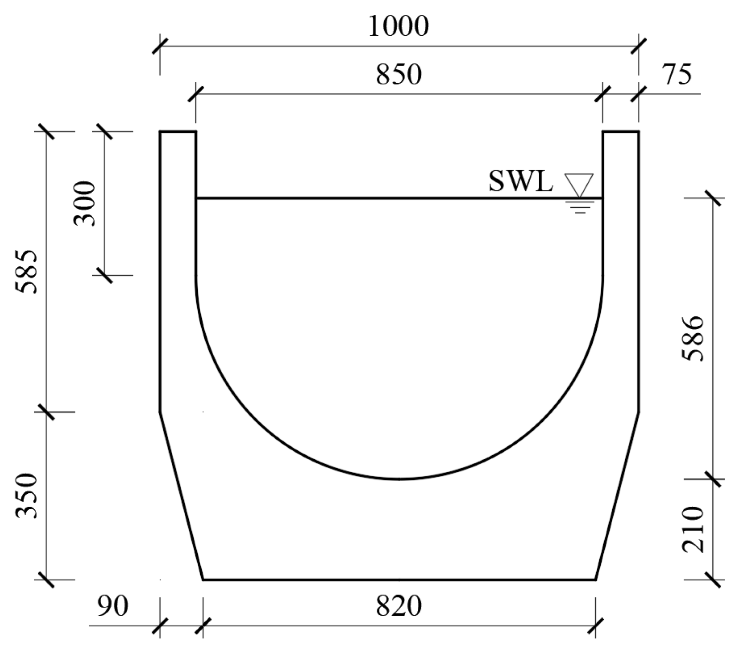
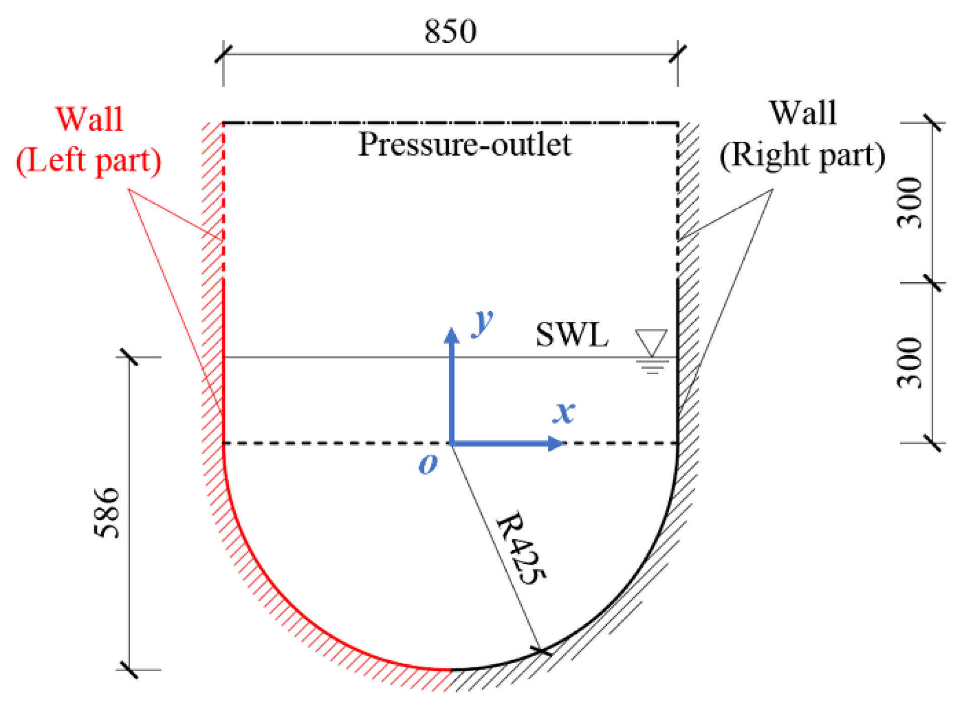
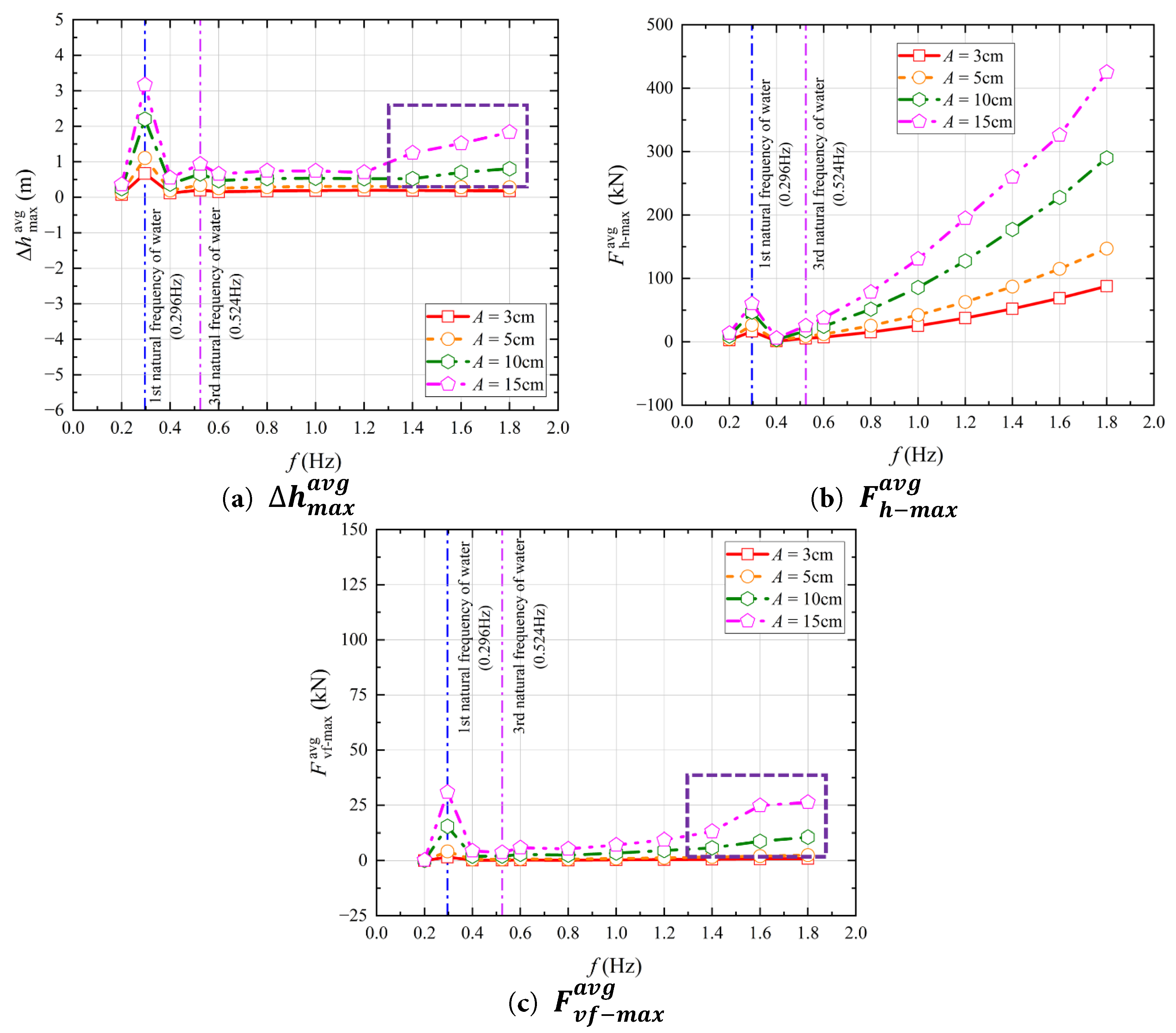
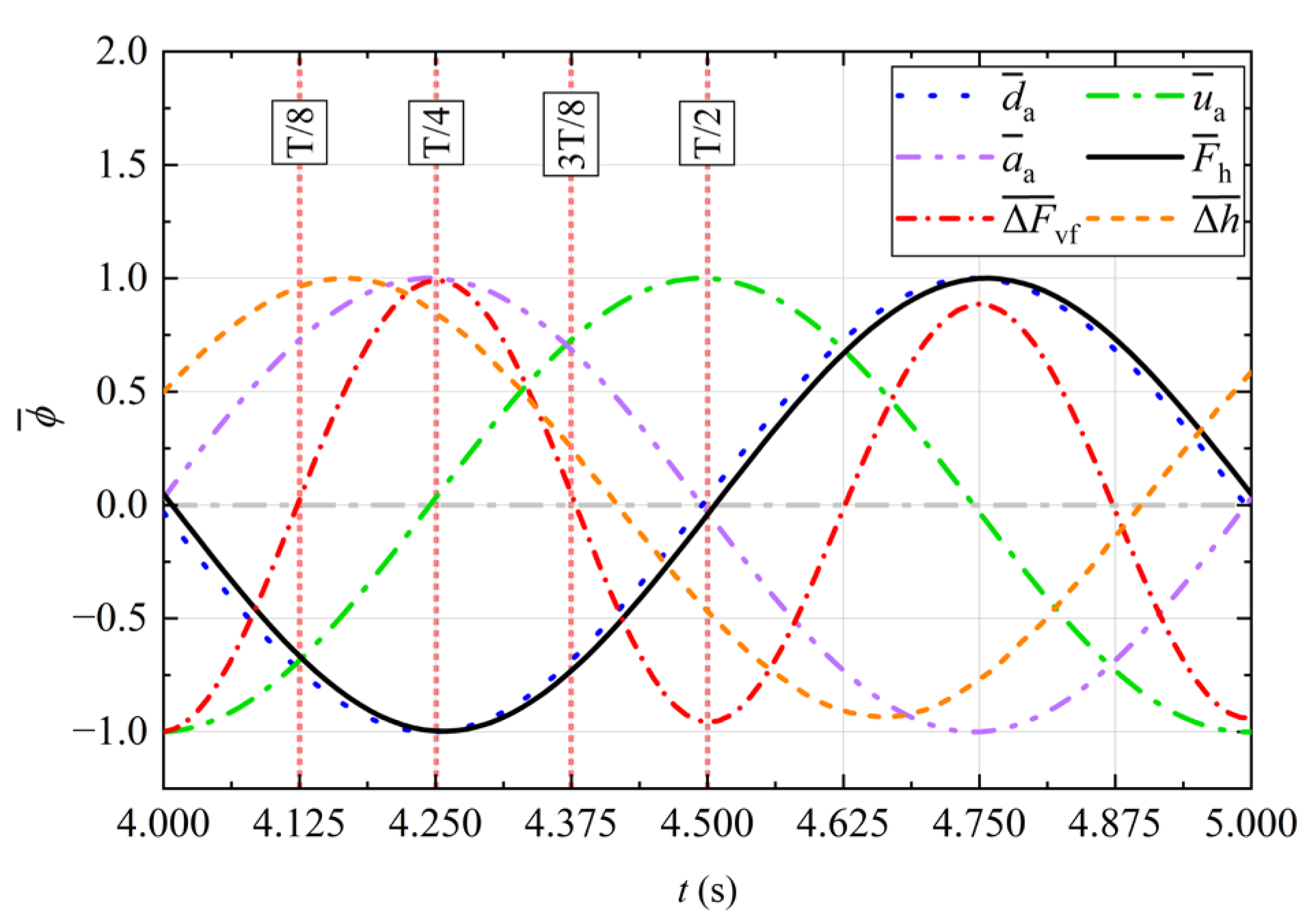
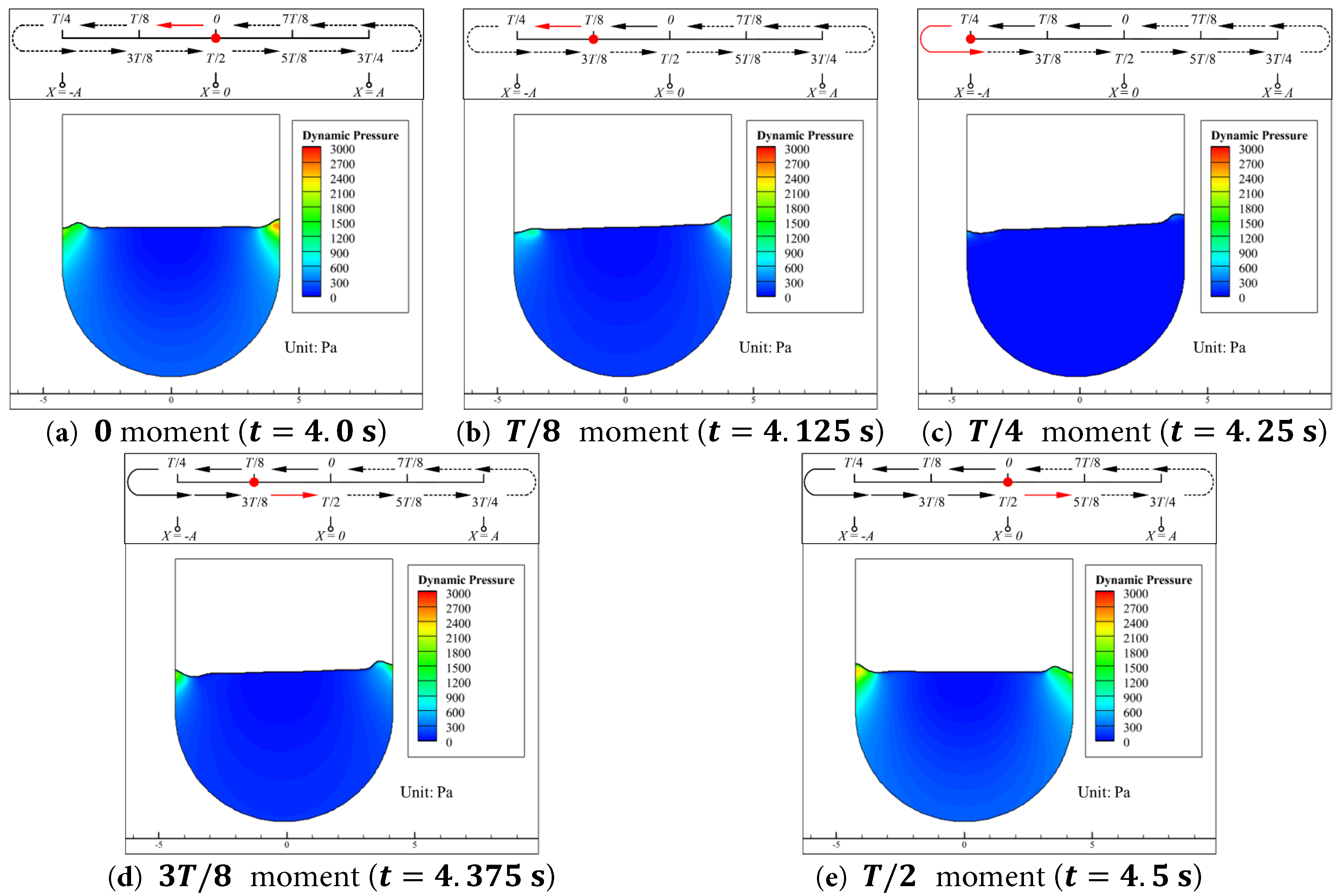
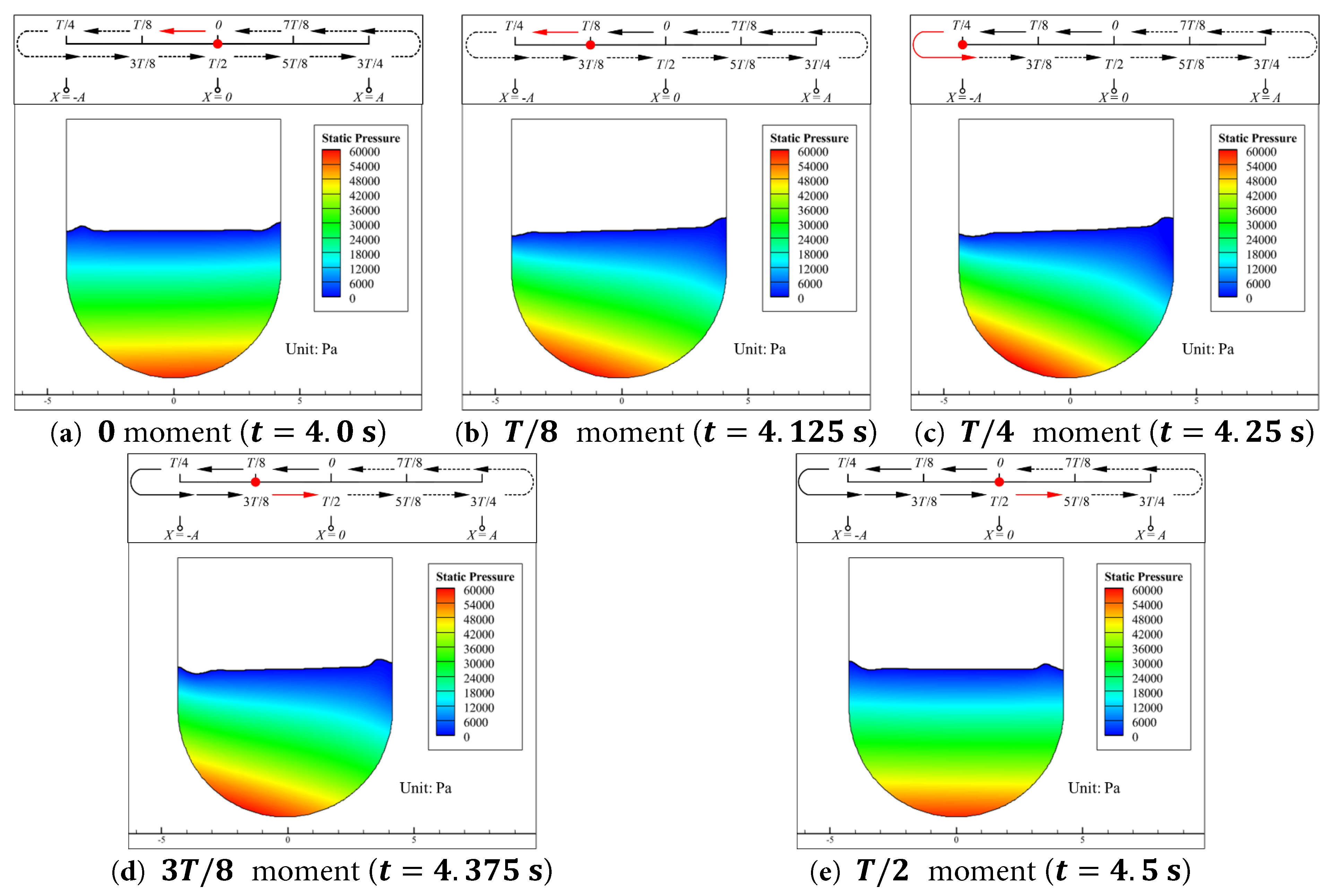
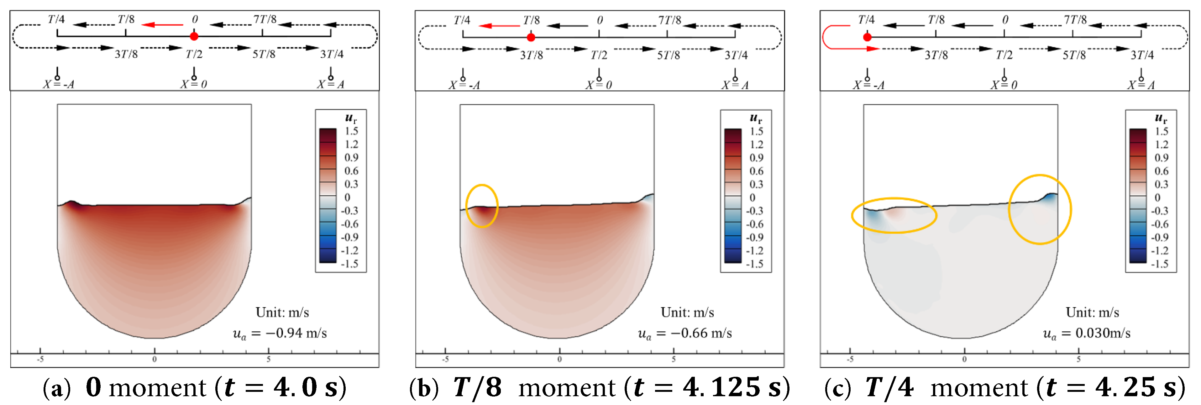
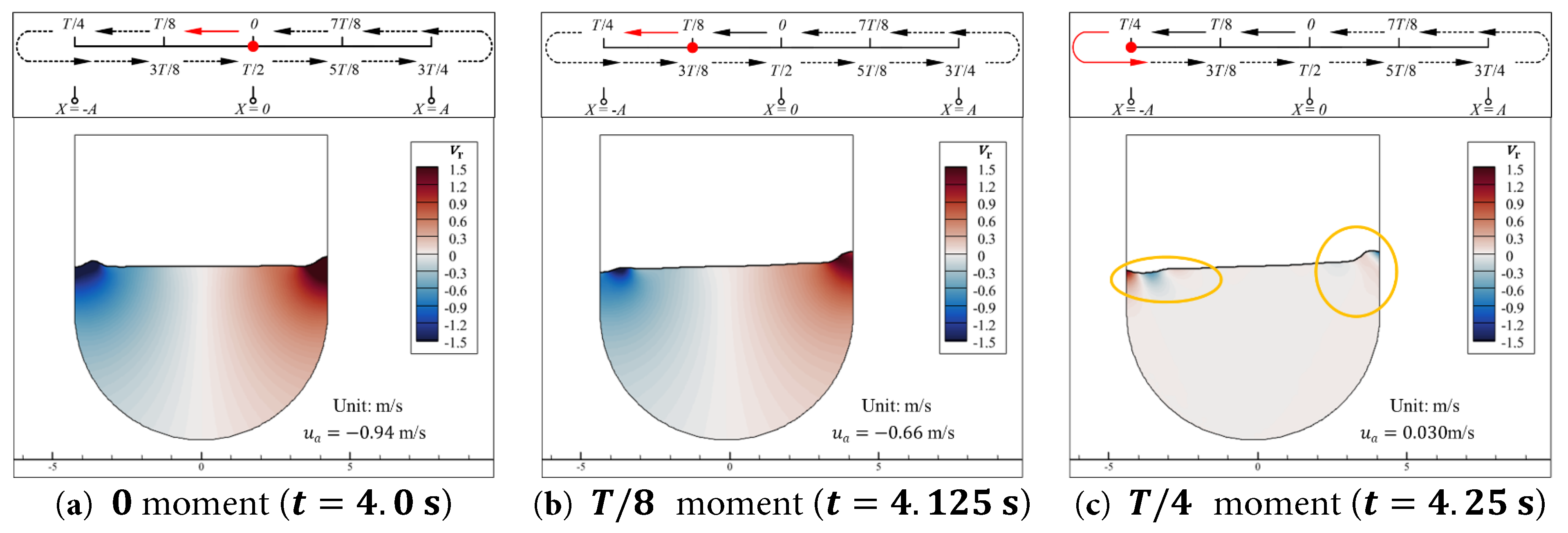
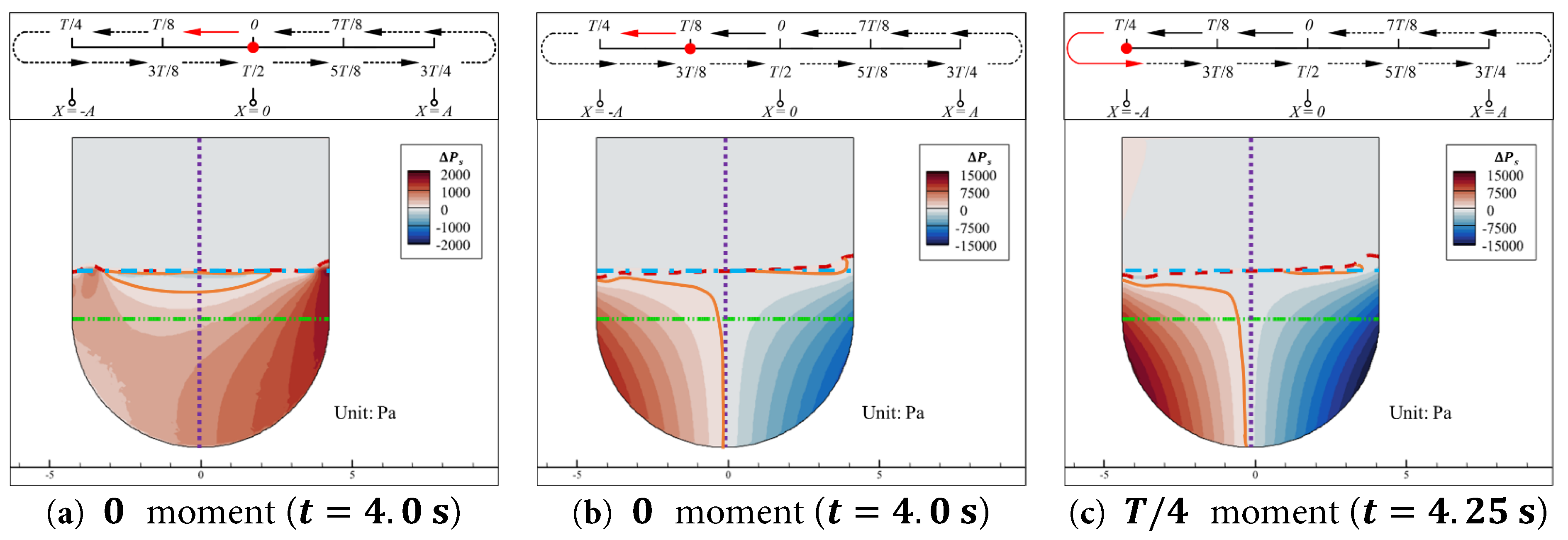
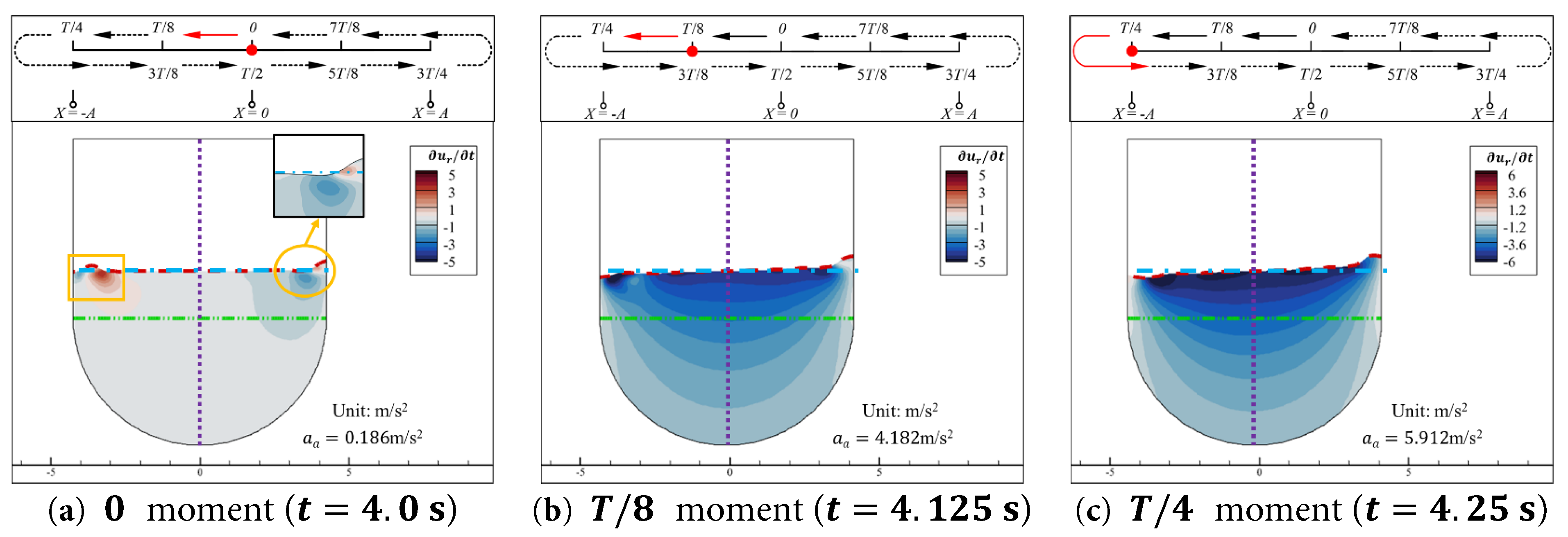
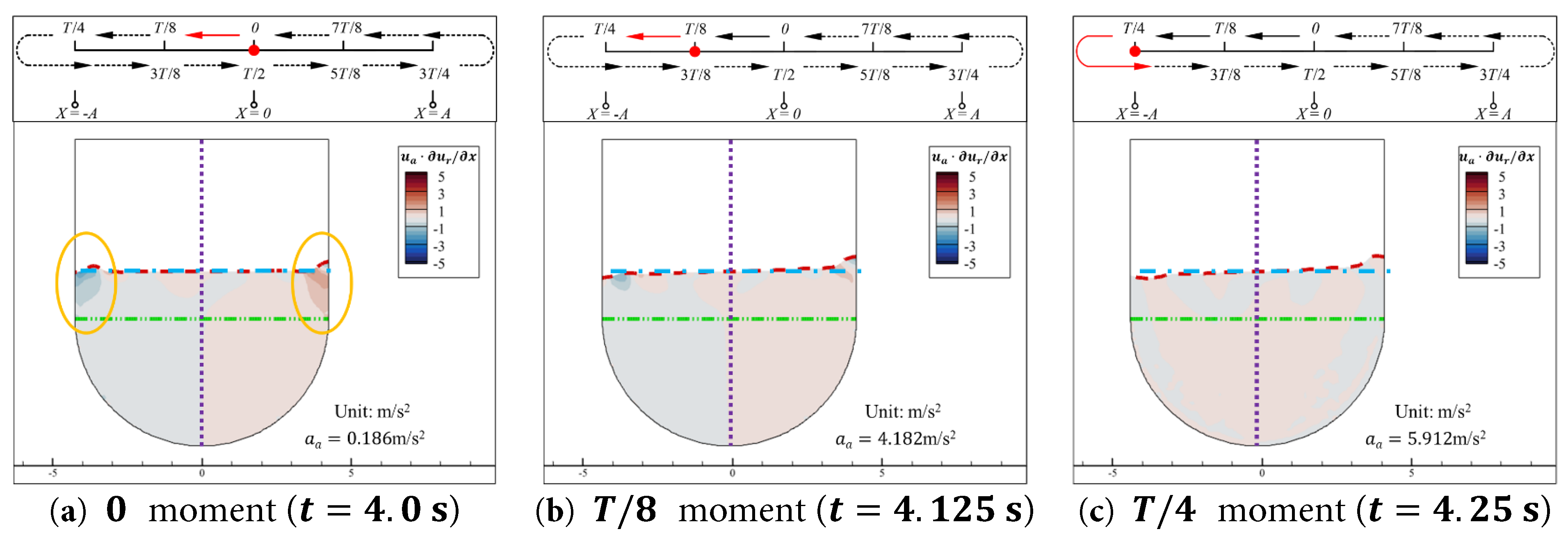
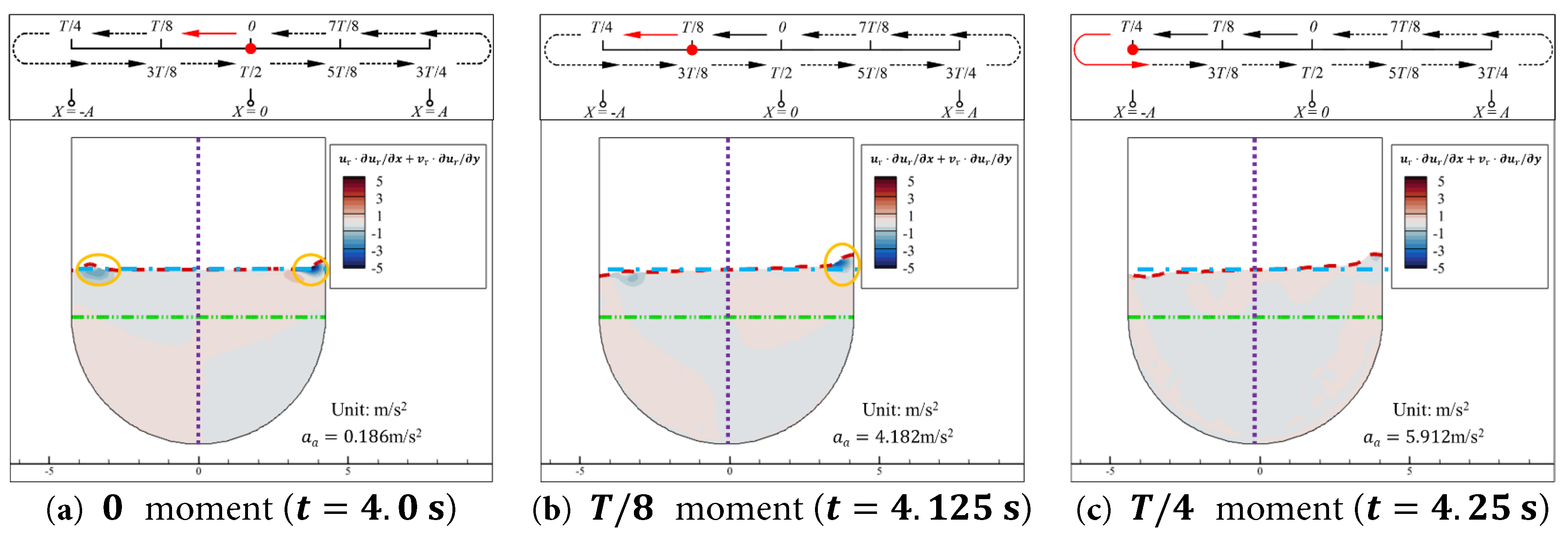
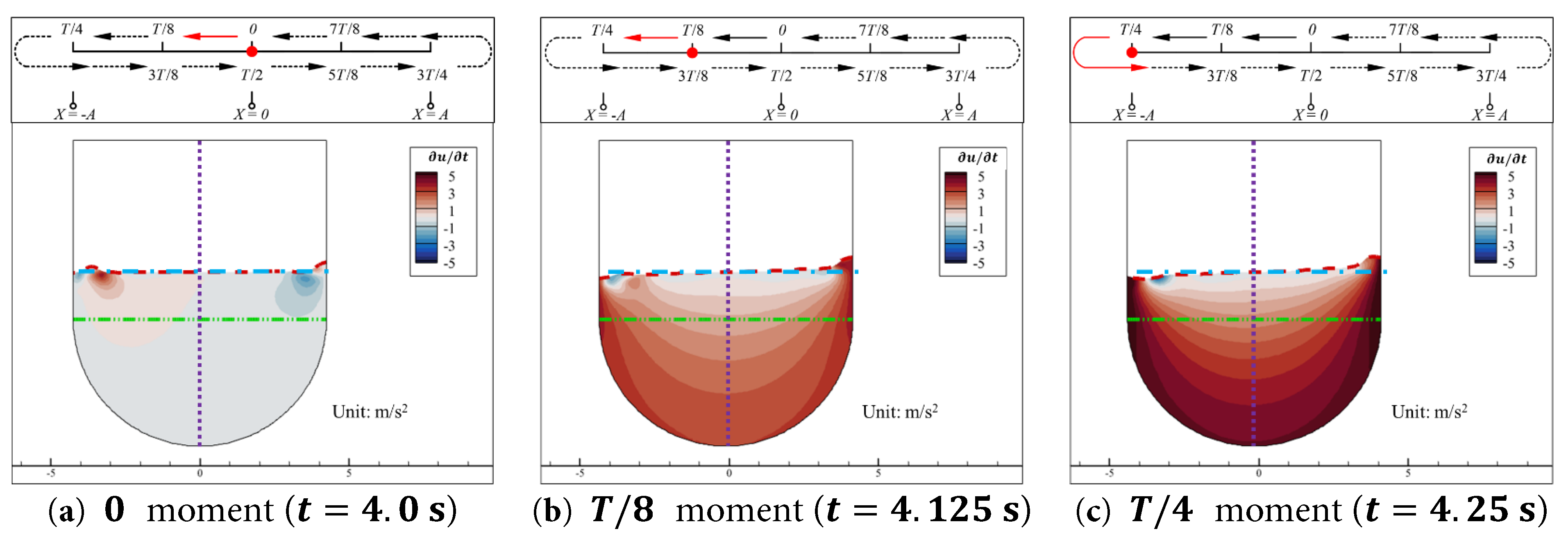
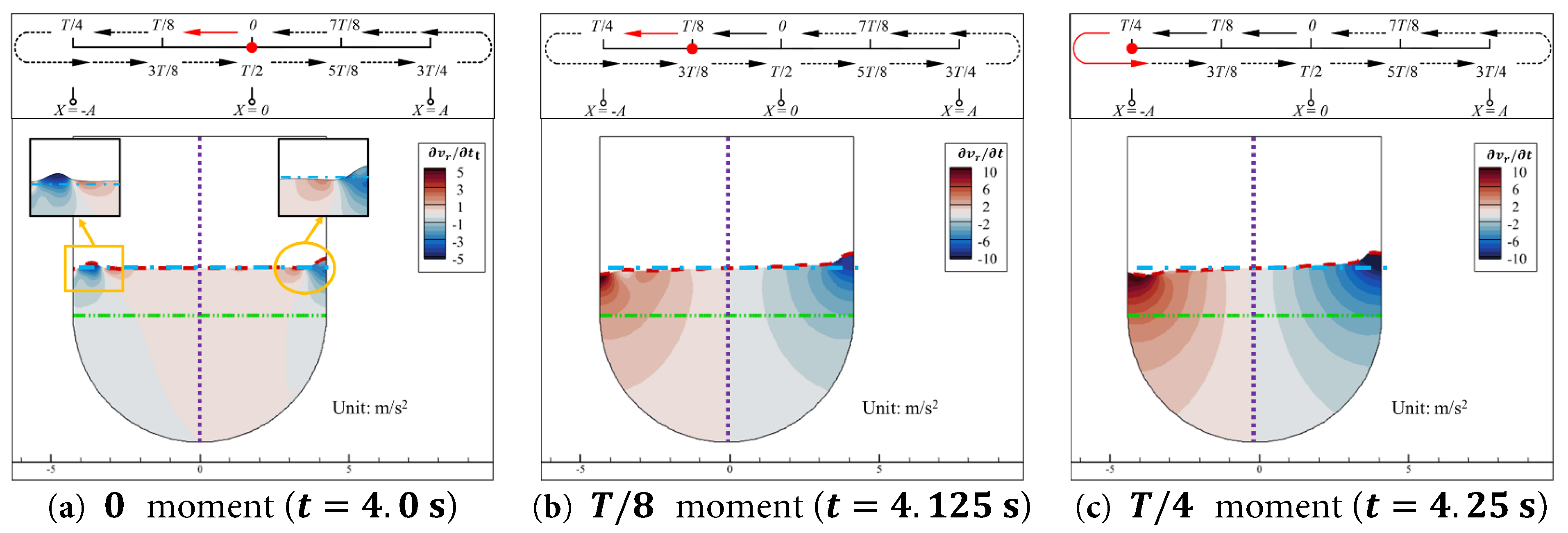
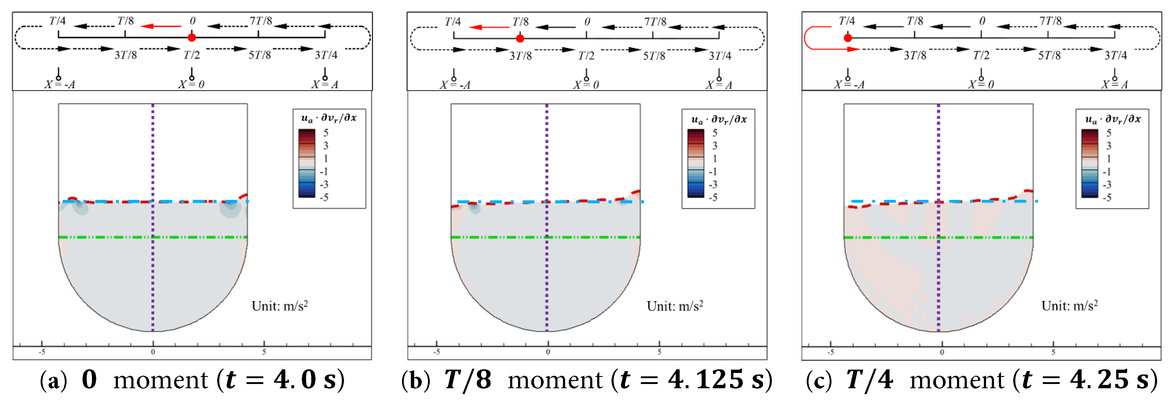

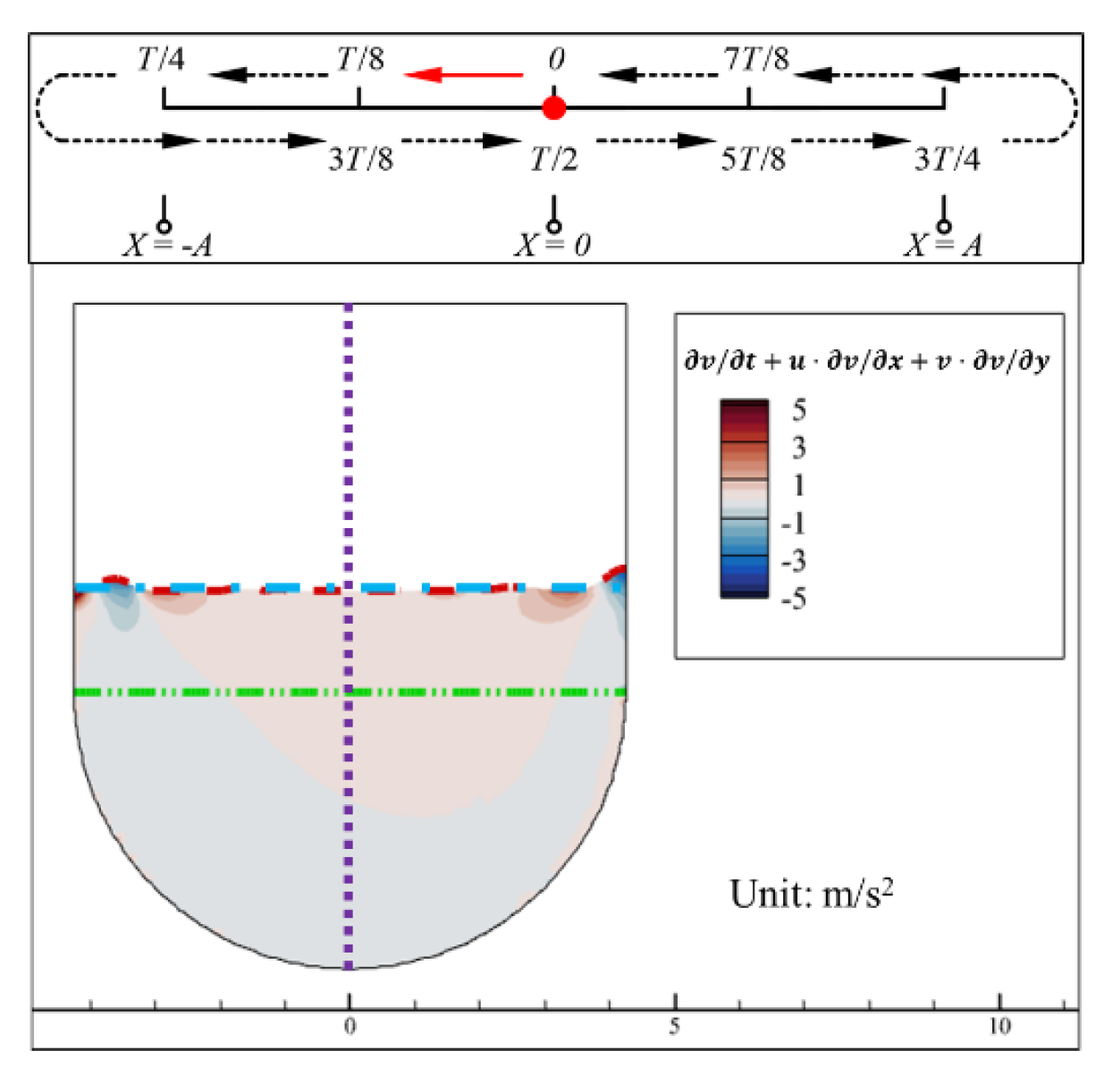

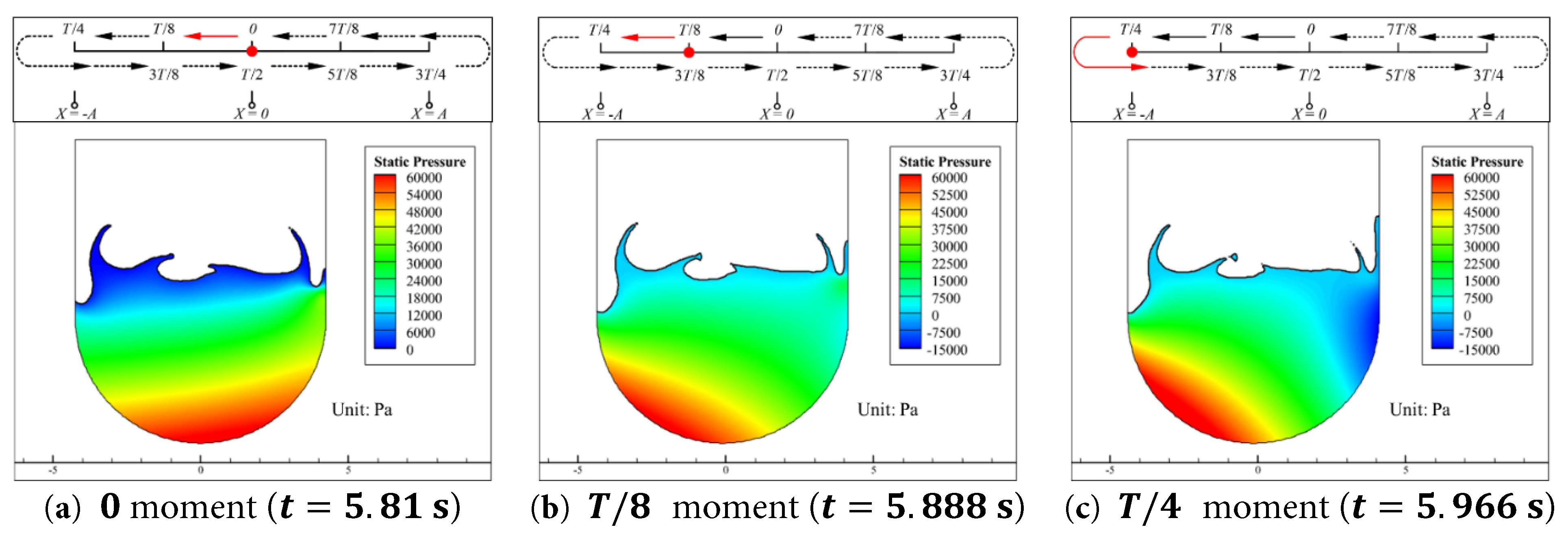
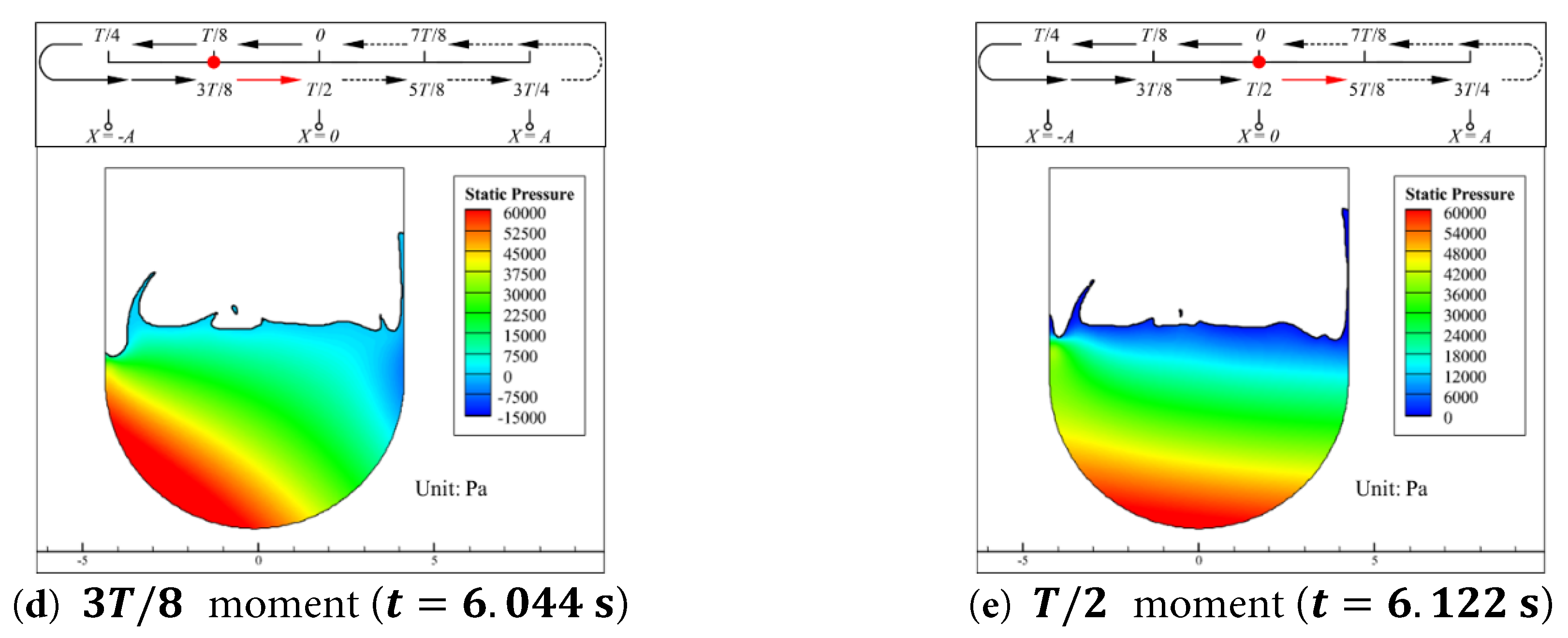
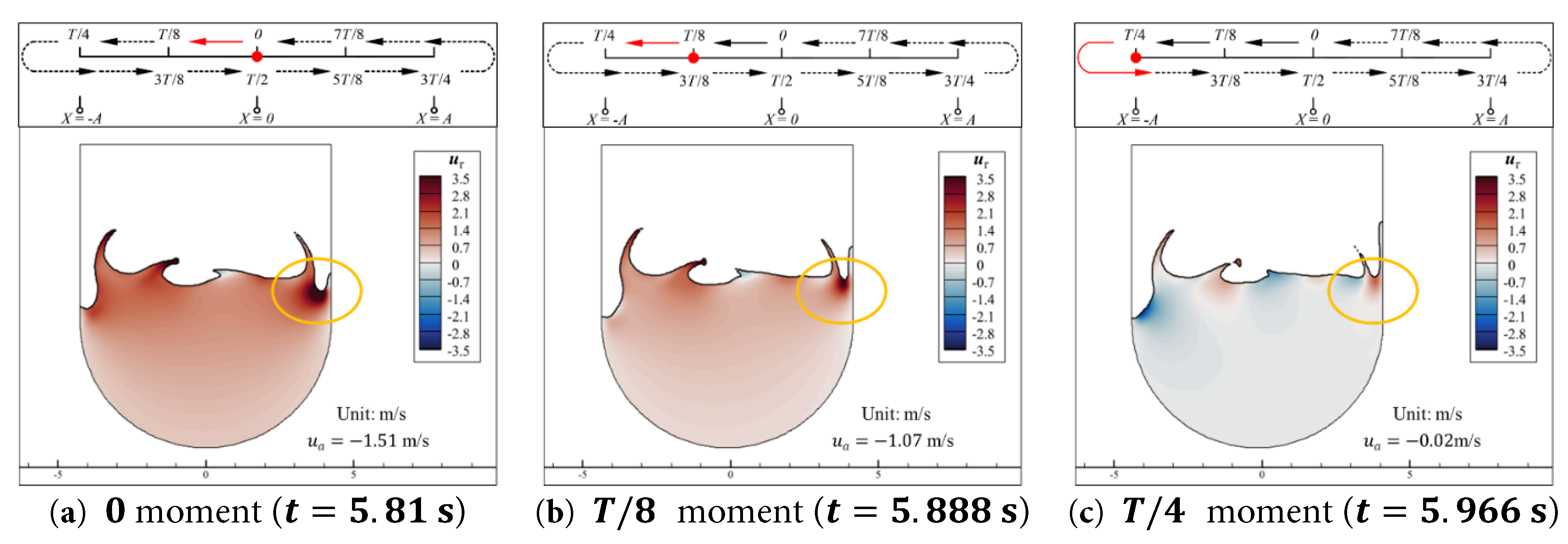
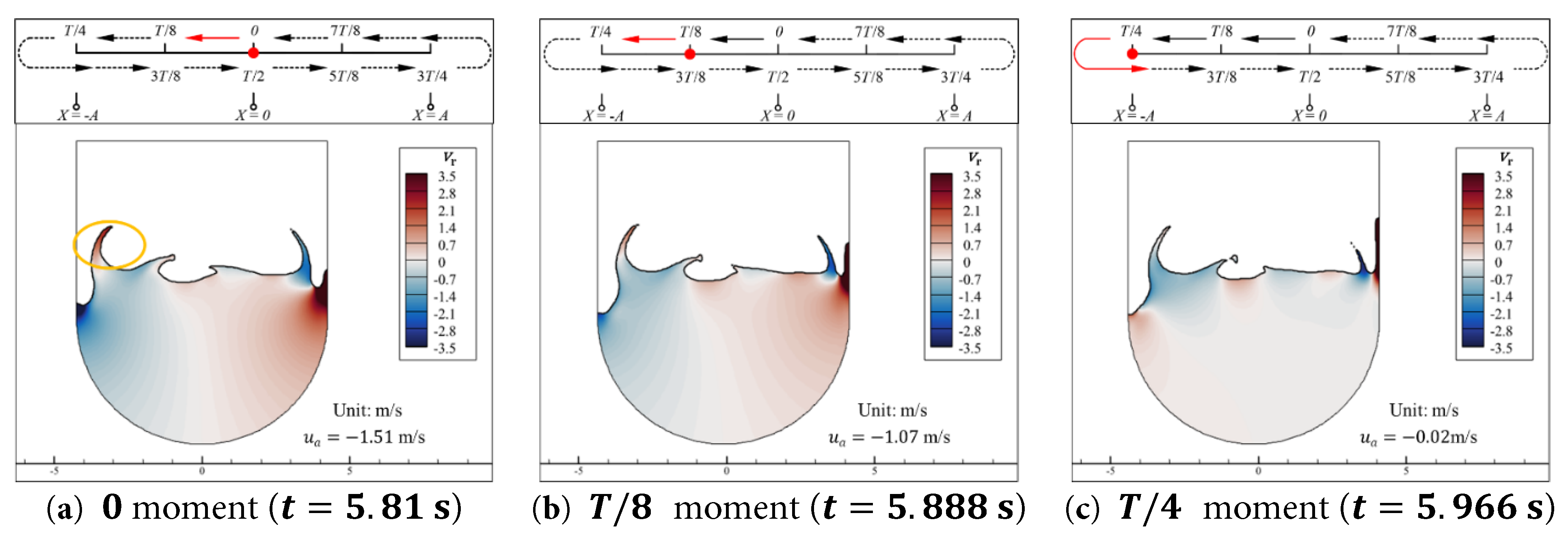
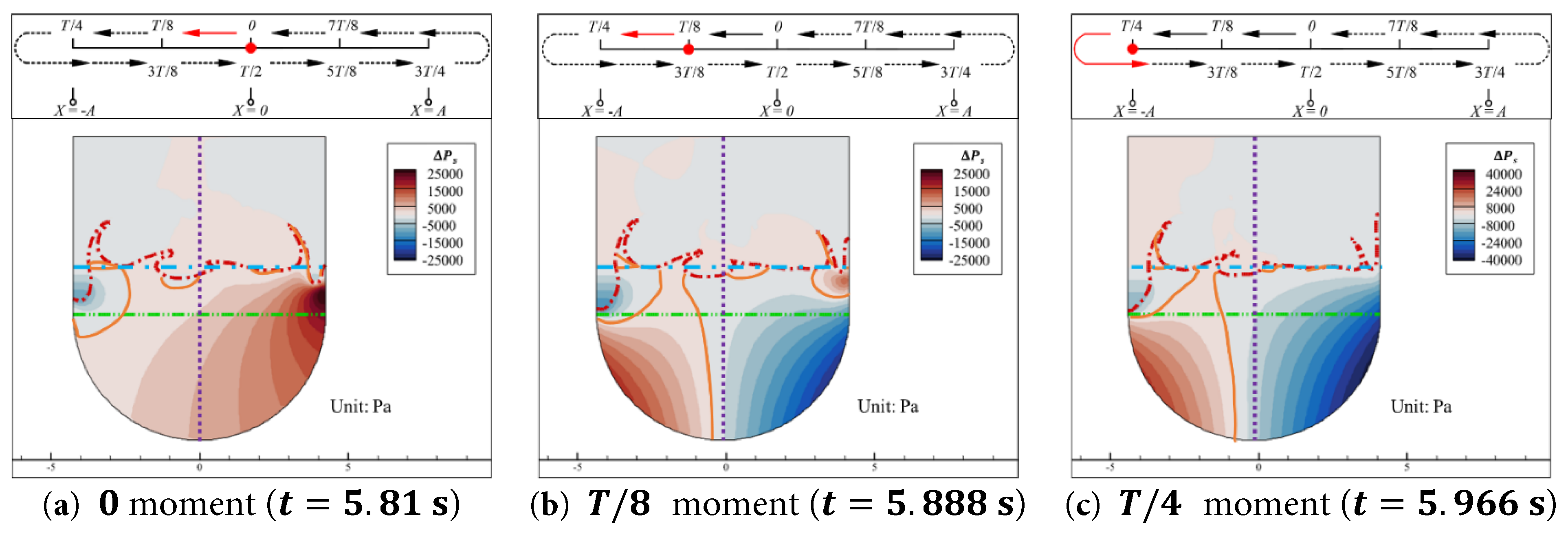
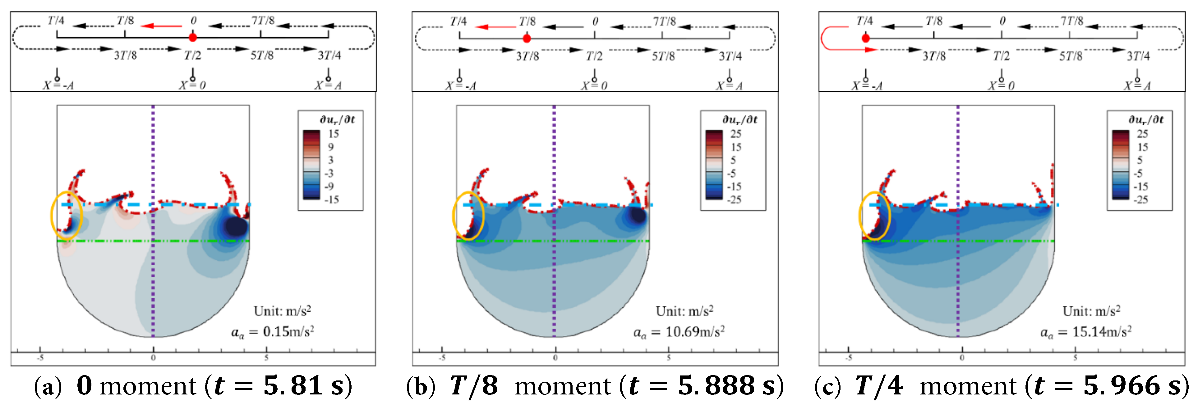
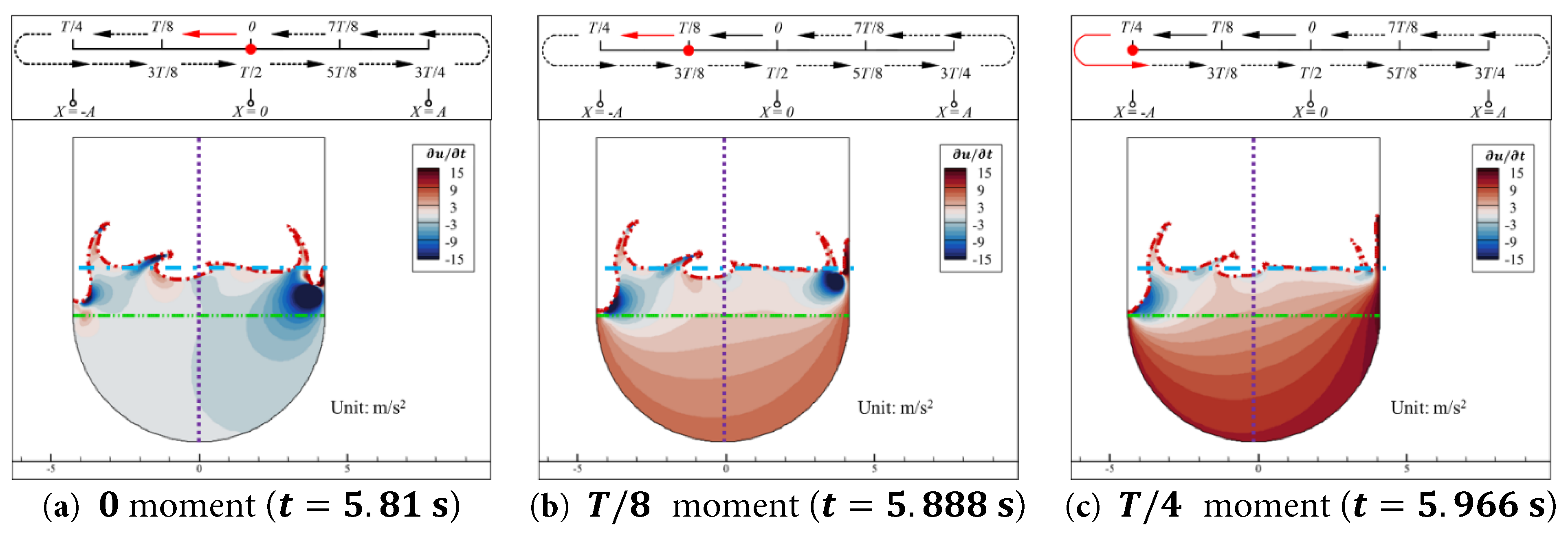
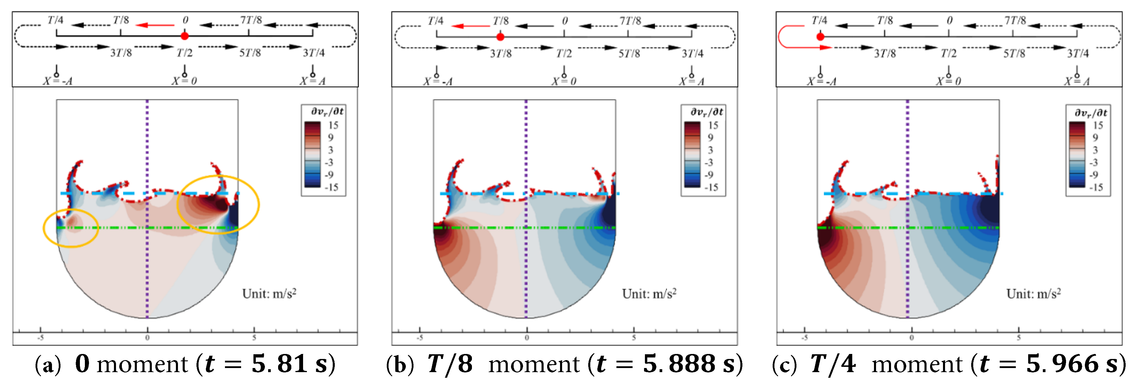
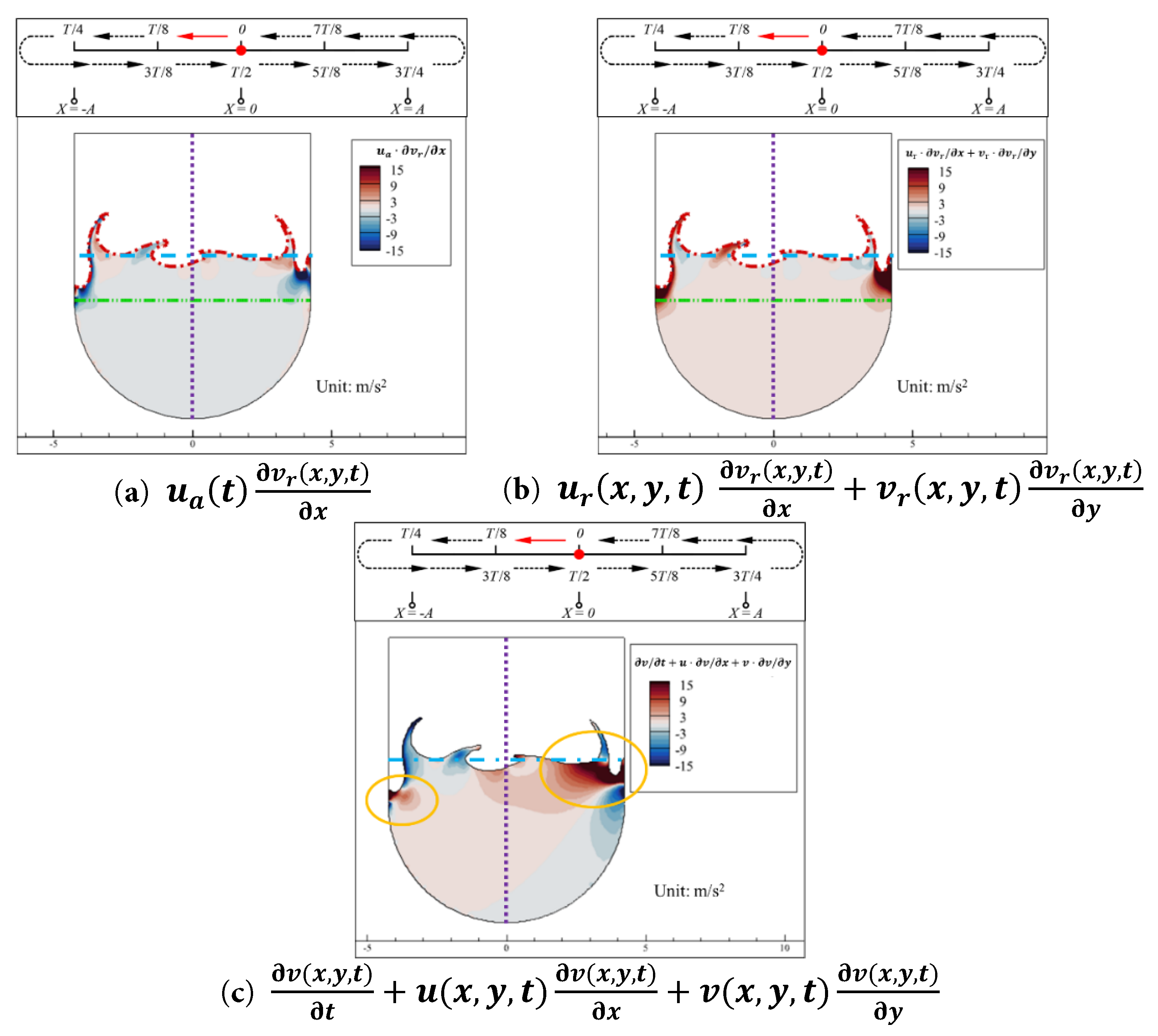
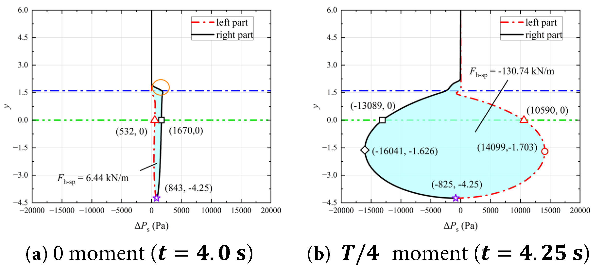
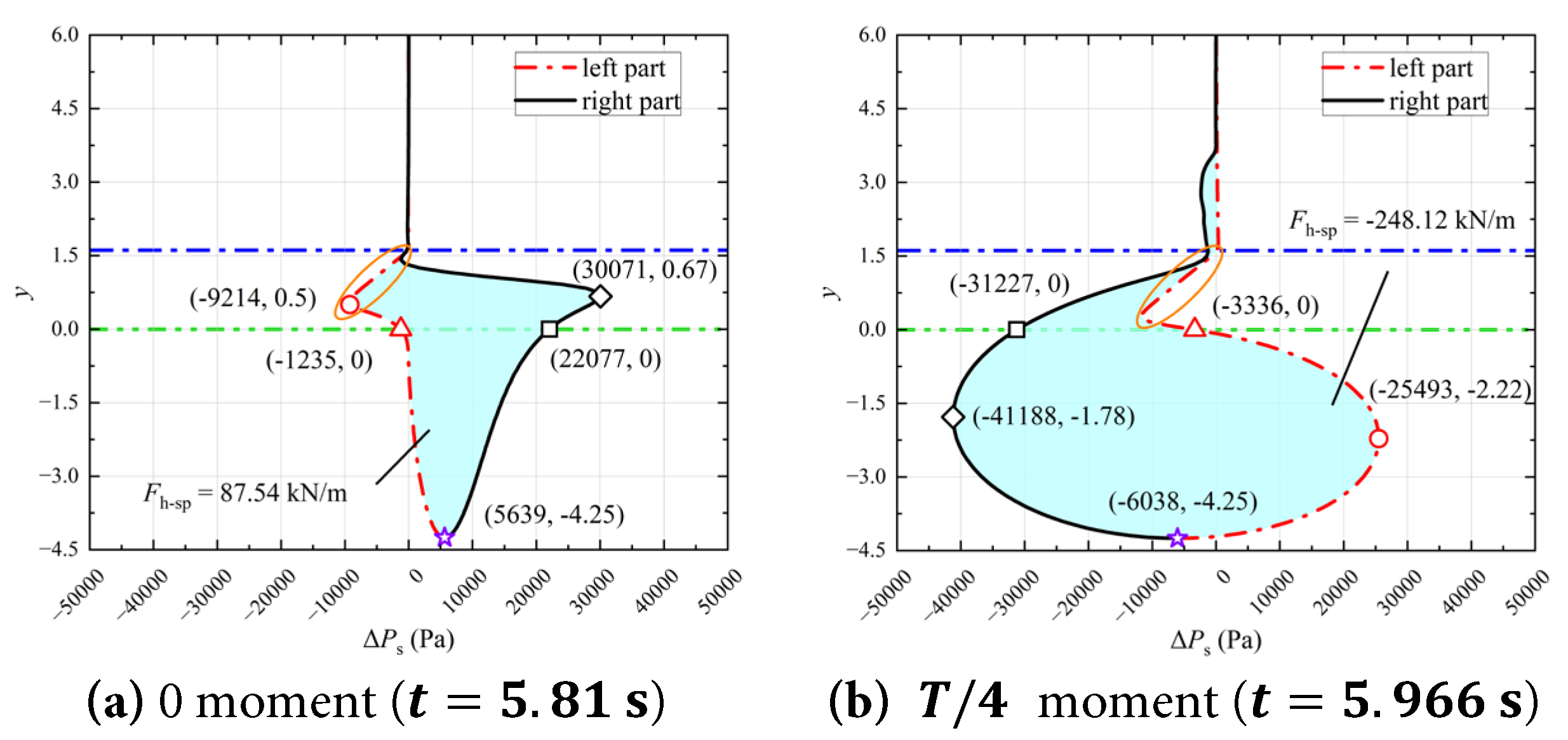
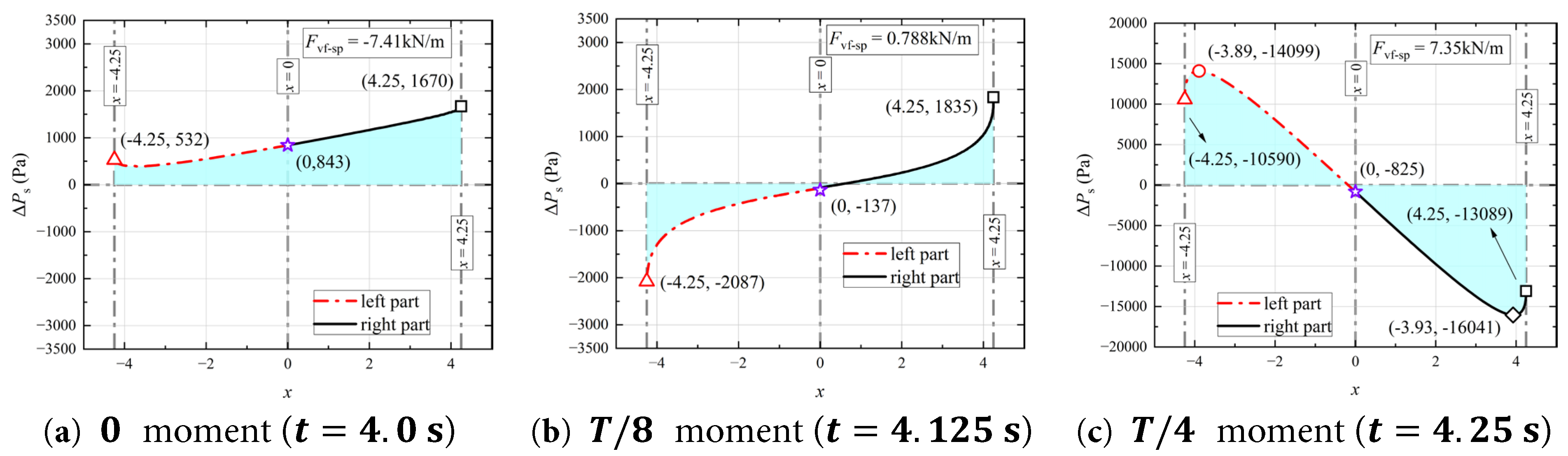
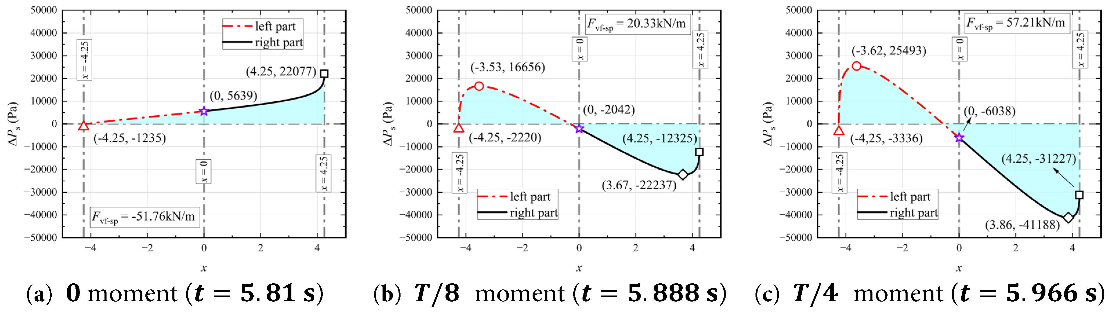
 Copyright © 2025 The Author(s). Published by Tech Science Press.
 Downloads
 Citation Tools