Optimization-Based Correction of Turbulence Models for Flow Prediction in Control Valves

1  Introduction

Control valves are critical pressure-regulating components in marine power systems, directly affecting vessel maneuverability and safety. Their role is to precisely adjust the flow rate, pressure, and direction of fluids within piping systems. Marine control valves are characterized by high-pressure differentials and high flow velocities, with internal flows exhibiting turbulent behavior, making accurate prediction challenging. Therefore, high-fidelity simulation of turbulent flow inside control valves is essential for the design and operational reliability of marine power systems. To address the limited accuracy of Reynolds-averaged Navier-Stokes (RANS) models in predicting turbulent flows within axial control valves, this study proposes a parameter optimization method for the SST k–ω turbulence model. By combining an artificial neural network (ANN) surrogate model with particle swarm optimization (PSO), our approach enhances the predictive capability of RANS simulations for such complex flows and provides more reliable computational tools to optimize the design of control valves in marine power systems.

With the development of computational fluid dynamics, the numerical simulation of the flow field prediction method for the control valve is becoming increasingly mature. Researchers have studied the numerical simulation of internal turbulence in control valve. Jin et al. [1] used the standard k–ε turbulence model and the mixture model combined with the Zwart-Gerber-Belamri cavitation model to clarify the internal flow and cavitation characteristics of the Sleeve flow regulating valve. Lin et al. [2] They designed two kinds of regulators to reduce the hydraulic impact. They studied the influence of the regulator on the hydraulic performance of the sleeve regulating valve in detail through CFD numerical simulation and experiment. Li et al. [3] optimized the structural parameters of the pilot-operated control valve based on CFD and orthogonal methods. The numerical simulation of three-dimensional flow in the valve is carried out by ANSYS CFX software, and the turbulence model is the SST k–ω turbulence model. Wu et al. [4] They compared and analyzed the regulating performance of the air-ring flow control valve and the central butterfly valve by numerical methods. The standard k–ε model in CFD is used to simulate the flow characteristics of the pipeline system. Tao et al. [5] studied the influence of V angle on the performance and internal flow characteristics of V-shaped ball valve and their relationship through experiments and numerical simulation. The realizable k–ε turbulence model is used to simulate flow characteristics. Singh et al. [6] investigated the flow characteristics of gas-liquid two-phase flow in severe-service control valves, with a focus on analyzing the effects of different valve openings (60% and 100%) and inlet gas volume fractions (5%, 10%, 15%) on flow behavior. The study revealed the non-uniform characteristics of the internal pressure field, phase velocity distribution, and void fraction within the valve. Additionally, the researchers quantified the interphase slip and flow asymmetry by defining the distribution parameter C0 and the local flow coefficient Kvrow.

Current research by scholars on the numerical simulation of turbulent flow in control valves primarily employs three methods: Reynolds time-averaged simulation (RANS), direct numerical simulation (DNS), and large eddy simulation (LES). DNS and LES are high-fidelity numerical simulation methods with high accuracy for turbulent flow prediction, but the calculation requires a lot of computing resources. Therefore, RANS is still the main simulation tool for turbulent flow [7,8]. RANS simulation relies on turbulence models to represent unresolved physical quantities. These models introduce great uncertainty into the results, seriously weakening their ability to predict complex flows, especially for the numerical calculation of turbulent flow inside axial flow control valves. The shear stress transport model (SST) is an all-round RANS model with excellent performance. It is also one of the best performance evaluations in the widely used eddy viscosity assumption turbulence model. It has the computational efficiency that DNS and LES cannot match and has a certain accuracy for the prediction of real flow. However, its eddy viscosity assumption for turbulence makes the empirical constants in the control equation need to be repeatedly verified with experiments to obtain [9,10]. As a result, default model parameters often fail to accurately predict flows in axial control valves due to their unique geometries and operating conditions.

In modern science and engineering, addressing multi-variable, nonlinear optimization problems presents a critical challenge, as traditional optimization methods often suffer from low efficiency and difficulty in guaranteeing global optimality. Recent advances in artificial intelligence have provided new approaches to solving such problems. Among these, artificial neural networks (ANNs) serve as powerful surrogate models capable of efficiently predicting system behavior by learning from historical data, while the particle swarm optimization (PSO) algorithm exhibits strong global search capabilities, making it highly effective for parameter optimization [11,12]. The integration of these two methods—hybrid ANN surrogate modeling with PSO—has emerged as a robust tool for tackling complex optimization problems. Zhang et al. [13] applied a BP neural network trained on CFD simulation data to study ejector cavitation, optimizing geometric parameters using PSO to effectively reduce cavitation-induced vibration while satisfying flow constraints. Qidwai et al. [14] focused on optimizing the positioning of micro-jet heat sinks, employing computational fluid dynamics (CFD) to generate training data for a radial basis function (RBF) neural network, which was then coupled with PSO to minimize thermal resistance. Their results demonstrated a remarkably low prediction error of just 0.56%. Additionally, Babanezhad et al. [15] combined PSO with a fuzzy inference system (FIS) (PSOFIS) to successfully predict the fluid velocity field in a bubble column reactor, achieving a superior regression coefficient (R = 0.98) compared to conventional adaptive neuro-fuzzy inference systems (ANFIS). This highlights PSO’s potential in complex flow modeling. These studies not only validate the feasibility of the ANN-PSO framework but also demonstrate its broad applicability in engineering practice. Compared with existing studies, the innovations of this paper are mainly reflected in the following aspects: (1) For the first time, the ANN-PSO hybrid algorithm is applied to optimize the parameters of the SST k–ω turbulence model for axial flow control valves, enabling data-driven automatic correction of empirical constants in the model; (2) An efficient collaborative framework integrating surrogate modeling and optimization algorithms is established, overcoming the inefficiency of traditional trial-and-error parameter calibration methods; (3) A specialized model correction scheme is developed for the unique operating conditions of high-pressure differential and high-flow-rate control valves in marine power systems, significantly enhancing the predictive capability of RANS models for such complex flows.

In summary, this paper proposes a novel turbulence model correction method based on an artificial neural network (ANN) surrogate model and particle swarm optimization (PSO) algorithm. This approach innovatively integrates data-driven modeling with intelligent optimization algorithms, achieving automatic optimization and calibration of empirical parameters in the SST k–ω model for axial flow control valves. Compared to conventional methods, the proposed approach not only enhances the accuracy and reliability of RANS turbulence models in predicting the flow capacity of axial flow control valves but also provides an efficient and intelligent new strategy for turbulence model calibration in complex engineering flow scenarios. This innovative methodology can be widely applied to the design and optimization of flow components in marine power systems and other industrial fields.

2  Axial Flow Control Valve Structure

The typical structure of an axial flow control valve is shown in Fig. 1, and its core components include valve body (1), anti-blowout gland (2), pinion shaft (3), noise reduction and pressure-drop assembly (4), locating sleeve (5), regulating spool (6), guiding assembly (7), support frame (8), rack shaft (9). The valve utilizes a gear-rack mechanism to achieve precise spool displacement control. Compared to conventional control valves, its innovation lies in the axial integration of the sleeve and spool within the valve cavity, thus ensuring that the medium flow direction remains stable. This unique structural design makes it a representative of energy-efficient control valves with outstanding advantages such as low flow resistance, large adjusting ratio, fast response, etc. It is especially suitable for critical areas such as naval power units.

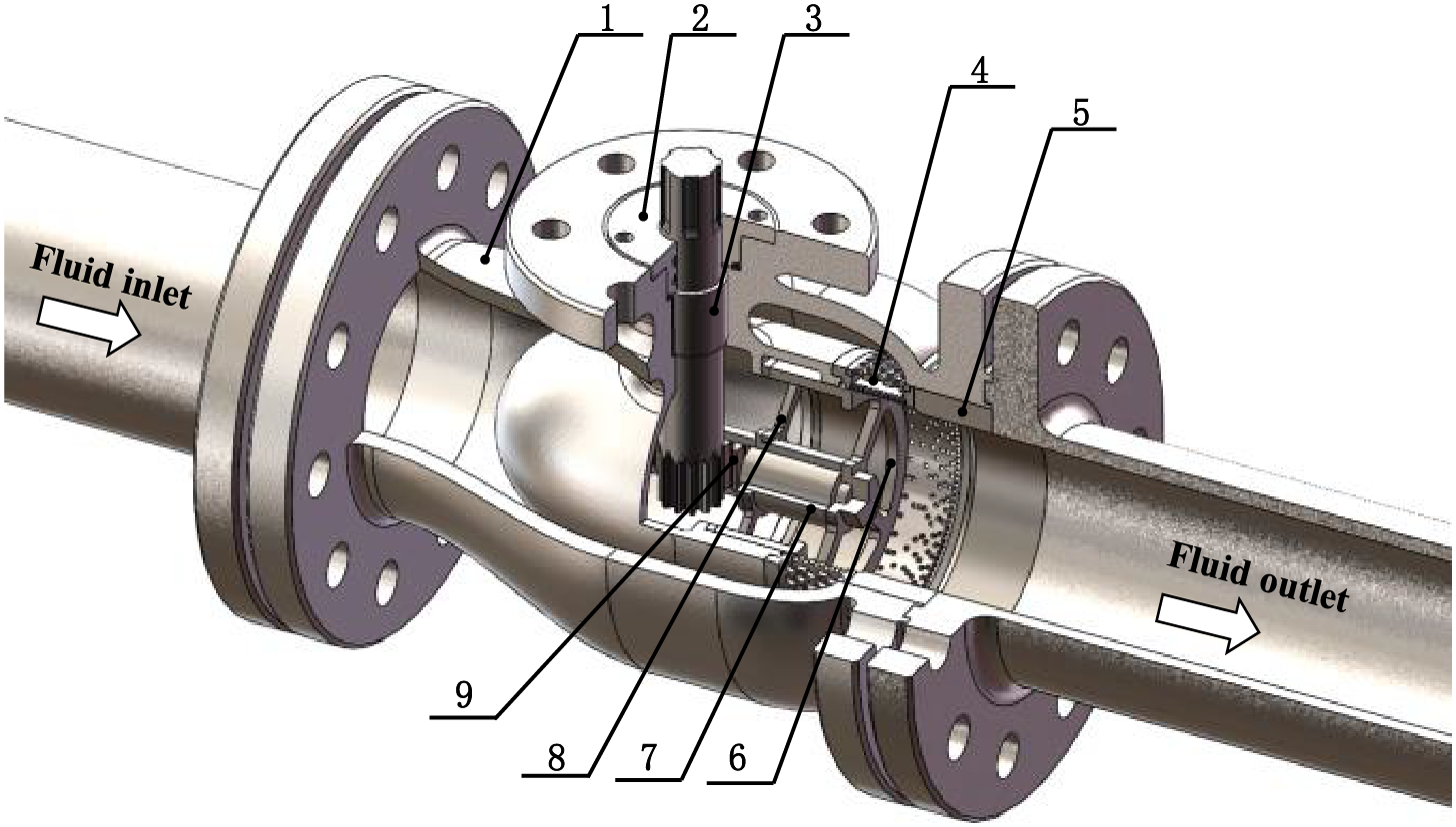
Figure 1: Local cutting of a three-dimensional model of the axial flow regulating valve

3  Numerical Simulation of Axial Flow Control Valve Flow

The flow behavior inside the axial flow control valve is analyzed using Computational Fluid Dynamics (CFD). The flow characteristics and flow capacity of the control valve are predicted by two CFD numerical simulation methods, SST k–ω, and LES, and compared and verified. By evaluating the flow coefficient curve and post-processing simulation data at varying valve openings, a detailed comparison of the internal flow patterns between the two methods is conducted.

3.1 Flow Channel Model Establishment and Mesh Generation

The geometrical model of the valve for multi-opening conditions was developed by 3D CAD software. To ensure flow development, the model incorporates 5DN upstream and 10DN downstream extensions. Under the premise of ensuring the accuracy of numerical calculation, the small structural features (e.g., process rounded corners, tiny chamfers, etc.) that do not affect the characteristics of the flow field are appropriately simplified, in order to improve the convergence rate of the calculation and to enhance the computational efficiency. Finally, based on the simplified geometric model, the fluid computational domain is reconstructed using the inverse modeling method, and its specific geometric configuration is shown in Fig. 2.

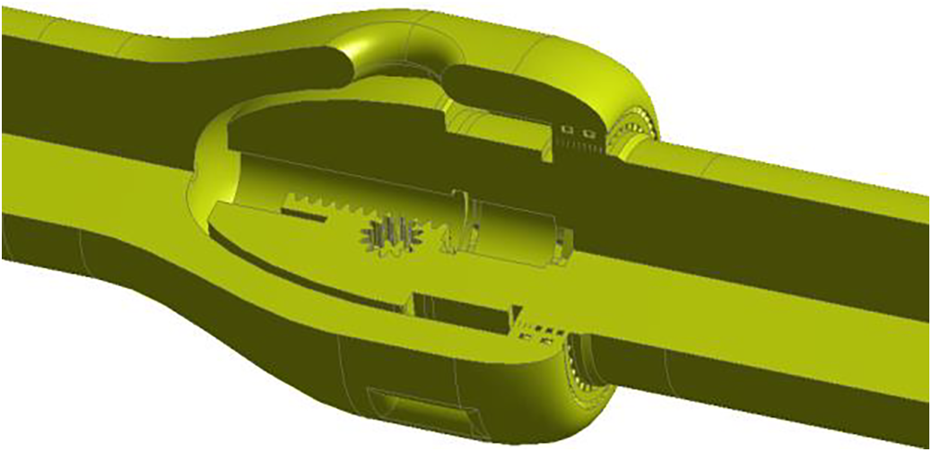
Figure 2: Flow channel model of the axial flow control valve

In this study, Fluent Meshing was employed to generate high-fidelity computational grids for the flow passage of an axial flow control valve. Based on flow characteristics, the valve passage was divided into three distinct regions, which are the straight pipe domain in front of the valve, Core regulation domain, and the straight pipe domain after the valve. A block-structured grid division is used for each region. The division of the overall flow channel grid and the sub-regional grid is shown in Fig. 3.

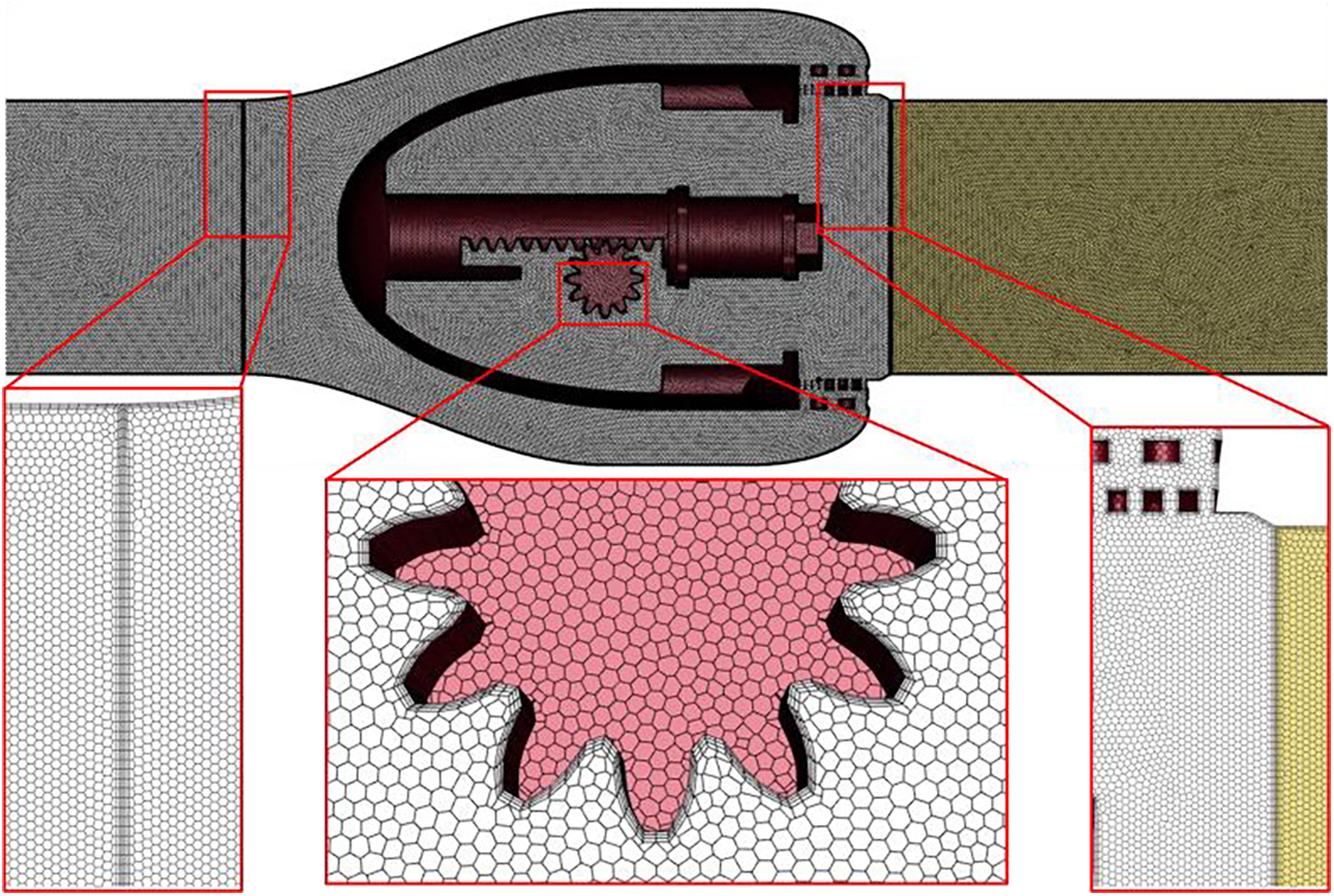
Figure 3: Overall grid division and local details of axial flow control valve

As shown in Fig. 3, adjacent mesh zones are connected through interface boundaries, with conformal mapping applied to polyhedral mesh interfaces to ensure node-to-node correspondence. By constraining the minimum geometric feature size, the overall fluid domain mesh achieves a smooth transition from fine to coarse scales, facilitating the generation of boundary layer grids across the entire domain to resolve near-wall flow characteristics. The boundary layer mesh employs a progressive refinement scheme, guaranteeing a y+ value below 1 in the near-wall region. Given that the most intense throttling process in the axial flow control valve occurs near the multi-stage pressure reduction assemblies, localized mesh refinement is applied to both the component walls and adjacent faces to capture critical flow features. Mesh quality in each region is assessed using maximum skewness and orthogonality metrics, complying with CFD simulation requirements of maximum skewness <0.95 and orthogonality >15°.

Fig. 4 presents the grid independence validation results for the flow characteristics of the fully open axial flow control valve.

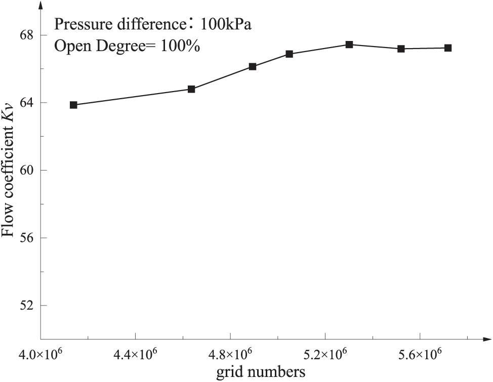
Figure 4: Grid independence verification

The grid independence study presented in Fig. 4 demonstrates that when the mesh count exceeds 4.6 million, a 16% increase in grid density results in merely a 2.3% variation in the flow coefficient (Kv). This marginal improvement in accuracy comes at the expense of substantially increased computational costs, indicating diminishing returns with further mesh refinement. Through localized grid refinement in critical regions, the selected 4.6-million-element mesh configuration proves sufficient to resolve essential flow characteristics while maintaining computational efficiency.

3.2 CFD Boundary Condition Determination and Solution Calculation

Numerical simulations were conducted in Fluent using a pressure-based solver with the SIMPLE algorithm. The Shear Stress Transport (SST k–ω) model and Large Eddy Simulation (LES) were adopted for turbulence modeling. Pressure inlet and outlet boundary conditions were applied, with a reference pressure of 1 bar. Surface roughness parameters were customized based on wall characteristics to improve accuracy. Spatial discretization employed the least squares cell-based method for gradients, second-order upwind scheme for pressure, and first-order upwind scheme for momentum, turbulent kinetic energy, and dissipation rate terms. Default relaxation factors were retained to ensure convergence.

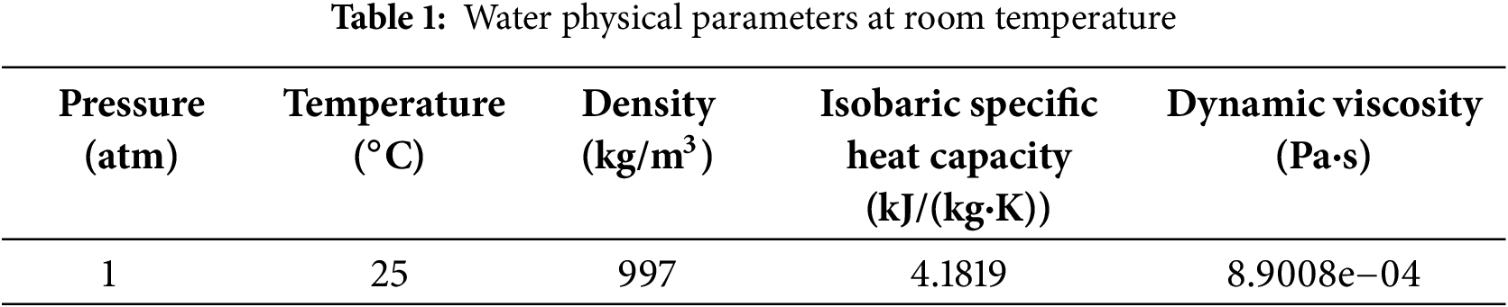
The convergence criteria during the solution process are: all normalized residuals (continuity, momentum, and k–ω turbulence equations) must fall below 1 × 10−6; with the valve outlet cross-section as the monitoring surface, when the fluctuations of the sliding average of the mass flow rate and the flow velocity at the centroid are not more than 1 ‰ in 50 consecutive iteration steps, the solution is considered converged. It should be noted that only the mesh types are different in the different discretization strategies, while the mesh sizes (including the body mesh size and the surface mesh size) are maintained identical. Simulations employed liquid water at 25°C (1 atm), with physical properties as specified in Table 1.

The SST k–ω and LES methods were used to simulate the flow values under three sets of pressure differences corresponding to each typical opening (10%, 20%, 30%, 40%, 50%, 60%, …, 100%). The pressure difference is set as shown in Table 2, and Fluent software is used to simulate the steady-state flow field under each typical opening.

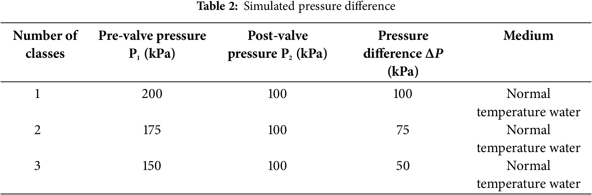
The arithmetic mean of the flow values simulated under the three groups of pressure differences is used to obtain the flow coefficient under the typical opening of the axial flow control valve. The three groups of different simulated pressure differences are shown in Table 2.

3.3 Comparison of Flow Characteristic Curves

The arithmetic mean value of mass flow under three groups of differential pressure is selected as the final mass flow of each typical opening. When the internal flow of the axial flow control valve is turbulent, that is, the Reynolds number Rev ≥ 10,000, the flow coefficient Kv of the axial flow control valve is calculated according to Formula (1), and the Reynolds number of the valve is calculated according to Formula (2).

Kv=10×Q×ρΔpv×ρ0(1)

Re=4×Qπdu(2)

In the formula, Q represents the volume flow of the measured medium water flowing through the axial flow control valve in unit time, unit m3/h; ΔPv represents the pressure difference at the pressure inlet of the straight pipe section before and after the axial flow control valve, unit kPa; ρ is the medium density, unit kg/m3; ρ0 is the density of water at 15.5°C, 999.1 kg/m3; d is the nominal diameter of the axial flow control valve, unit m; u is the kinematic viscosity of water, unit m2/s.

According to the results of SST k–ω simulation and LES simulation, the flow coefficient values of the axial flow control valve under typical opening (10%, 20%, 30%, 40%, 50%, 60%, … , 100%) are calculated, respectively. The flow coefficient Kv of the axial flow control valve is calculated according to Formula (1). The calculation results of the two simulation methods are shown in Table 3.

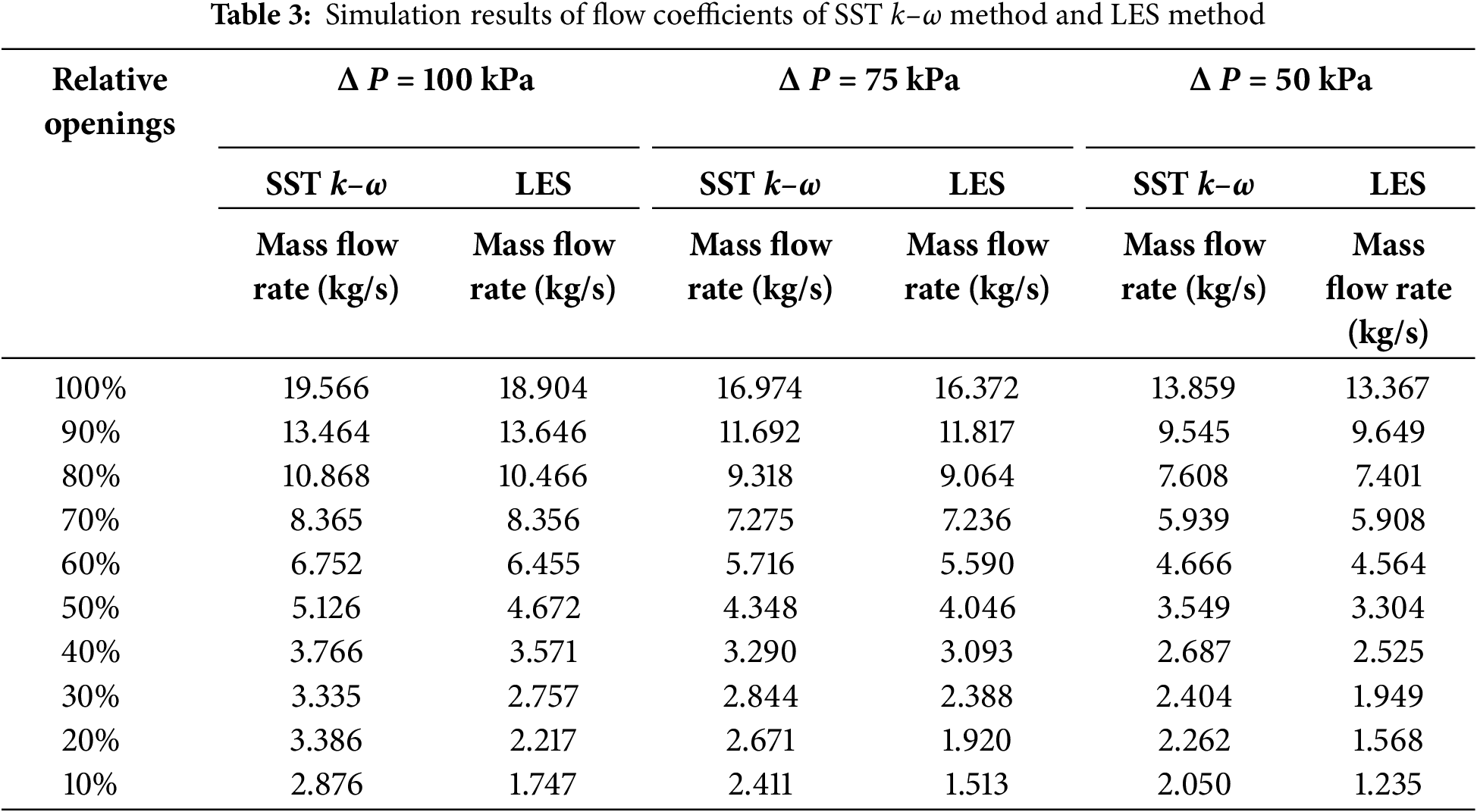
According to the numerical simulation results of the two simulation methods in Table 3, the flow characteristic curve of the control valve is fitted, and the results are shown in Fig. 5.

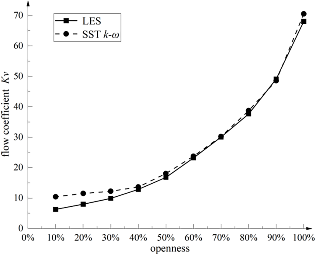
Figure 5: The axial flow control valve flow characteristic curve

It can be seen from Fig. 5 that when the axial flow control valve is above 50% opening, the results of SST k–ω simulation and LES simulation are similar. When the opening is below 50%, the SST k–ω simulation results gradually deviate from the LES results, and the SST k–ω simulation accuracy decreases at a small opening. The axial flow control valve adopts a multi-stage depressurization structure, and it is necessary to verify and optimize its depressurization performance and air defense capability at a small opening. According to the LES simulation results, the empirical coefficient of the SST k–ω turbulence model at a small opening can be corrected, so that the prediction of the axial flow control valve is closer to the simulation results of the large eddy simulation, but the calculation amount is still maintained at the Reynolds average level. The discrepancies observed in Fig. 5 stem from fundamental differences between the SST k–ω and LES approaches. The SST k–ω model, as a Reynolds-averaged method, relies on empirical coefficients to represent turbulence effects, leading to smoothed predictions of flow separation and pressure recovery-especially at small openings where complex vortices dominate [16]. In contrast, LES resolves large-scale turbulent structures directly, capturing transient flow details but at a prohibitive computational cost [17]. This trade-off between accuracy and efficiency motivates the turbulence model correction in Section 4.

3.4 Comparative Analysis of Internal Flow Field

From the flow characteristic curves of the axial flow control valve, it can be seen that there is a large deviation between the large eddy simulation LES and the prediction of the SST k–ω turbulence model at the small and maximum openings. The flow condition at 10% small opening of the axial flow control valve is selected for analysis. Since the flow inside the axial flow control valve is symmetrical, the internal flow field is analyzed in the horizontal direction. A comparison of the pressure cloud information on the horizontal cross-section inside the 10% opening of the axial flow control valve for the two different simulation methods is shown in Fig. 6.

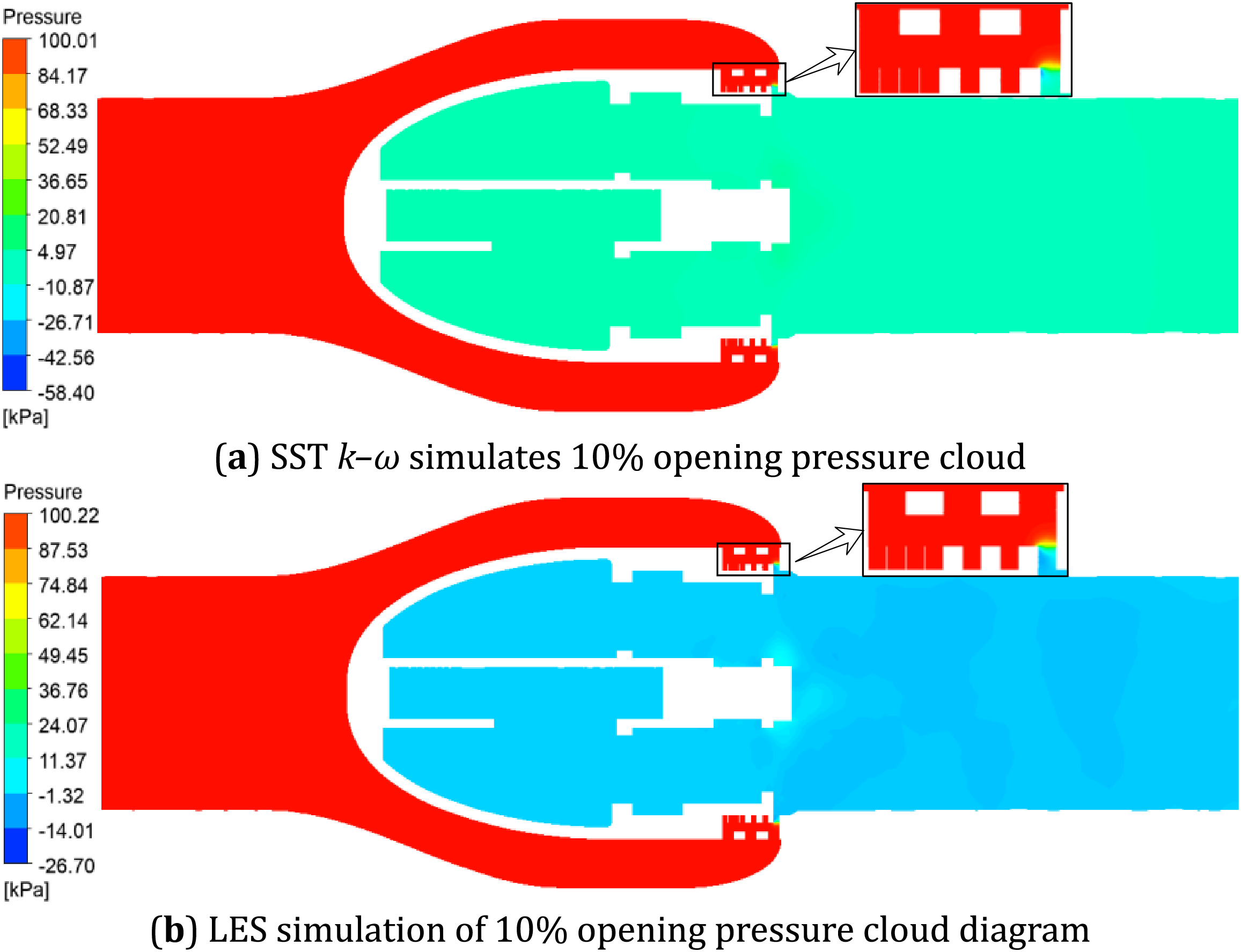
Figure 6: Comparison of pressure contours between SST k–ω simulation and LES simulation at 10% opening

From the pressure distribution cloud diagram of the axial flow control valve at 10% opening obtained by the SST k–ω simulation method in Fig. 6a, it can be seen that due to the change of opening, the orifice of the two-layer throttling sleeve is closed by the valve core and cannot flow through the fluid. The fluid is filled with the gap between the two layers of the pressure-reducing sleeve. The throttling is accomplished through the remaining orifice, and the fluid experiences a sharp acceleration in the narrow gap, resulting in a significant drop in static pressure from the inlet 100 kPa. In contrast, the LES large eddy simulation results in Fig. 6b show a finer flow structure, and the LES prediction results show a more uniform pressure distribution behind the valve with a predicted value of 5 kPa, which is 50% different from that of the SST results; moreover, the pressure gradient changes more gently, and the pressure restoration process, especially in the throttling region, is closer to the physical reality. This difference mainly stems from the limitation of the SST model to simulate complex separated flows with high Reynolds numbers, whose default turbulent dissipation coefficients are too high, leading to an underestimation of the flow energy loss. This also explains the significant deviation of the flow coefficients of the two methods in the low-opening zone in Fig. 5.

Two different simulation methods of axial flow control valve 10% opening of the internal horizontal section of the velocity contour information as shown in Fig. 7.

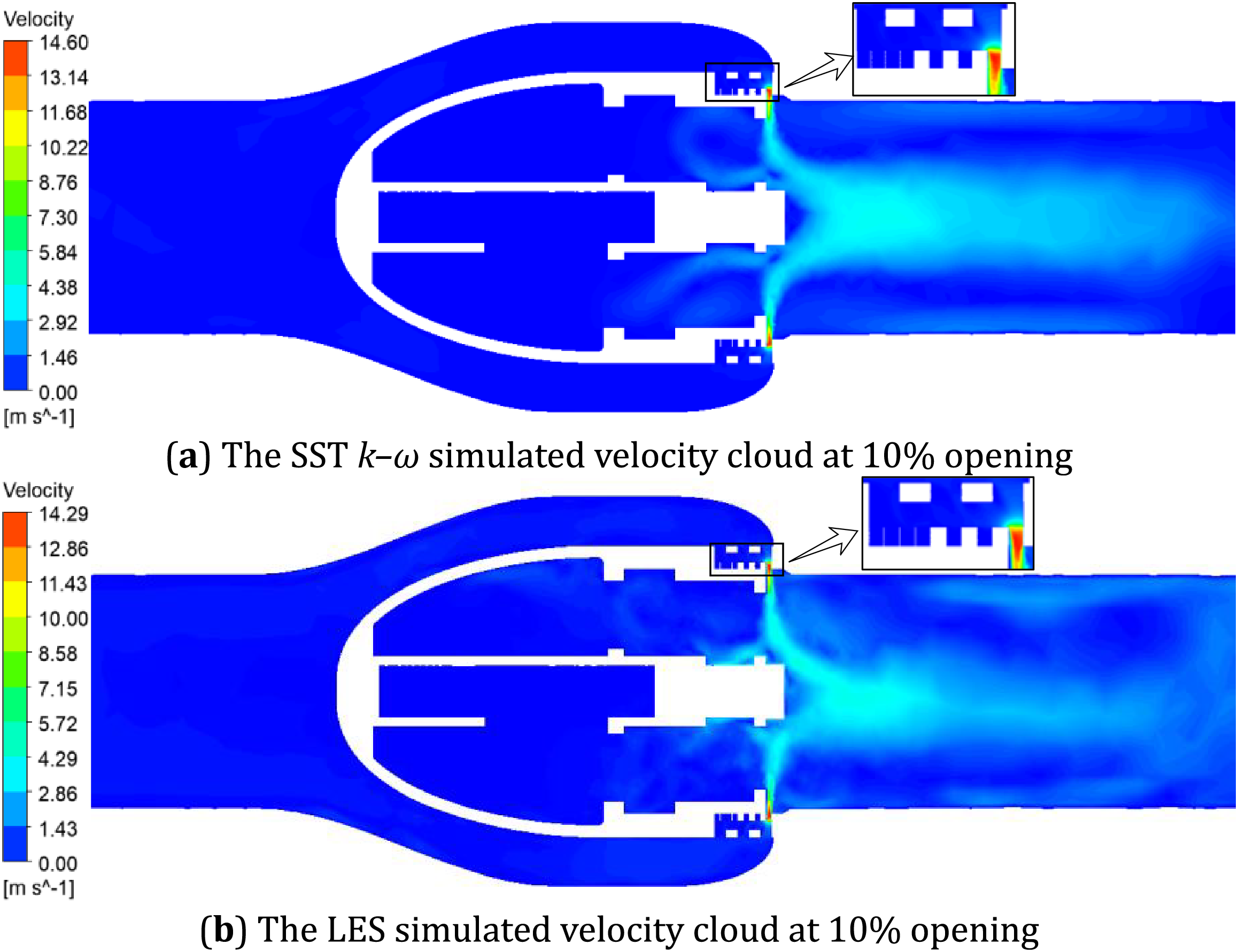
Figure 7: Comparison of velocity cloud between SST k–ω simulation and LES simulation at 10% openness

The velocity distribution program of the axial flow control valve under 10% opening obtained by the SST k–ω simulation method is shown in Fig. 7a: Due to the change of the opening degree, the position of valve core and transmission component changes, the high-speed fluid after the sleeve throttling converges around the transmission rod, the speed decreases rapidly, presenting a smooth axisymmetric jet. Since the SST k–ω model is based on the Reynolds-averaged formulation, it is unable to resolve the transient secondary vortices generated by flow separation, predicts a smaller recirculation zone.

The velocity distribution cloud diagram of the axial flow control valve under 10% opening obtained by the LES simulation method is shown in Fig. 7b: After the opening changes, the position of the valve core and the transmission component changes, and the high-speed fluid velocity after the sleeve throttling decreases rapidly, presence of a significant low velocity recirculation zone. Comparing Fig. 7a with Fig. 7b, it can be seen that the speed behind the 10% opening valve predicted by SST k–ω simulation is about 3.65 m/s, which is about 0.2 m/s faster than the speed behind the valve obtained by LES simulation.

A comparison between Figs. 6 and 7 reveals that the simulation results obtained by the SST k–ω method differ from those of the LES large eddy simulation, which is recognized to have a higher simulation accuracy. In the region of straight pipe sections where the flow is simple, the simulation results for both are approximately the same. However, there is a large deviation in the simulation results at the multi-stage pressure-reducing sleeve, which may be due to the complex structure of the pressure-reducing sleeve of the axial flow control valve. The high Reynolds number flow and the dispersion and aggregation of the fluid occur here, resulting in the prediction accuracy of the SST k–ω method is not as good as that of the LES large eddy simulation method. To verify this idea, the simulation results of a complete depressurization route at the multi-stage depressurization of the horizontal section of the axial flow control valve SST k–ω and LES are monitored. The middle line of the distance between the two stages of the step-down sleeve is taken as the origin, and the direction of the fluid flow is taken as the positive direction. The schematic diagram of the monitoring line position at 10% opening is shown in Fig. 8.

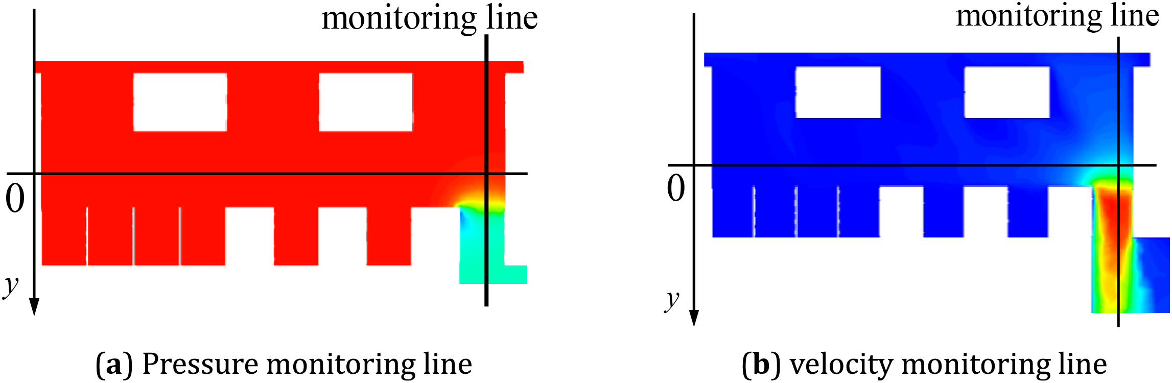
Figure 8: 10% opening monitoring line position diagram

The comparison of the monitoring results of the two simulation methods is shown in Fig. 9.

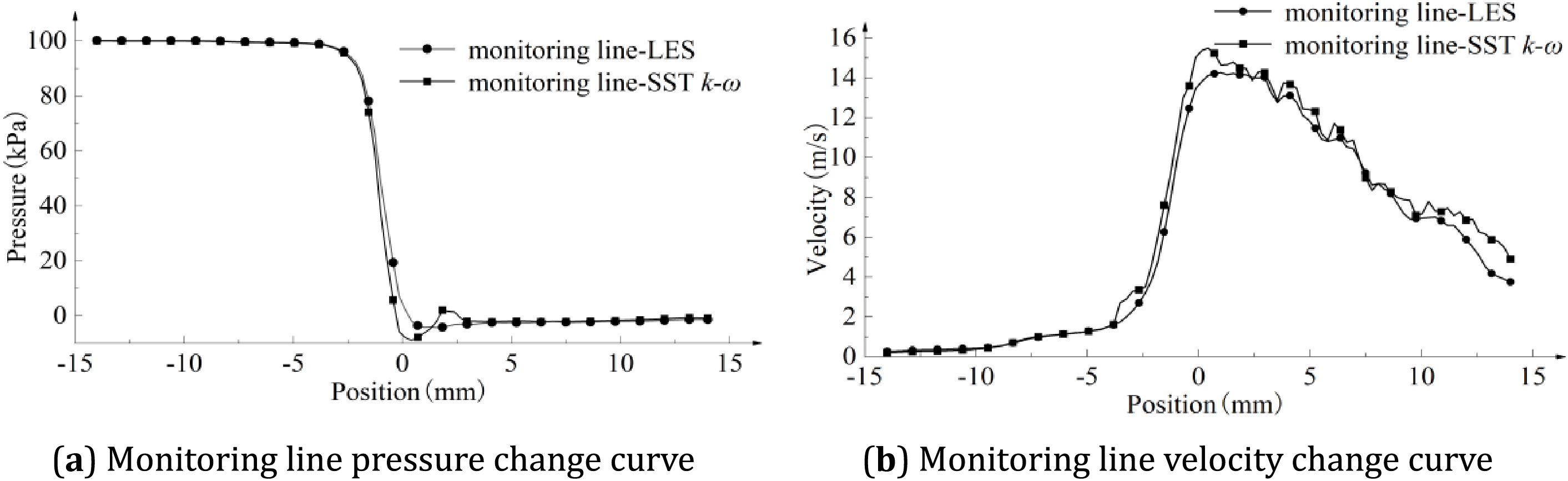
Figure 9: 10% opening SST k–ω simulation and LES simulation pressure and velocity monitoring

As shown in Fig. 9a, the pressure change curve on the monitoring line at 10% opening is shown, and the center section of the two-stage pressure-reducing sleeve is at the coordinate 0 point. The results of the two simulations are different near the coordinate 0 point, and the trends and values of the other positions are comparable. As shown in Fig. 9b, the velocity change curve on the monitoring line at 10% opening is shown. After throttling, the prediction results of the two begin to differ significantly. The main manifestation is that the simulation results of SST k–ω are numerically higher than those of LES simulation results, and the trends are roughly the same.

According to the comparison of the simulation results of the axial flow control valve SST k–ω simulation method and the large eddy simulation LES method, according to the pressure and velocity distribution of the internal flow field, and the comparative analysis results of the pressure and velocity change curves on the monitoring line: The predicted value of the axial flow control valve flow based on the RANS SST k–ω turbulence model at small opening is different from the simulated value obtained by the large eddy simulation LES. The specific performance is the same in the trend, but the maximum difference in value is about 7.6%. To ensure the accuracy and economy of the CFD numerical simulation of the control valve and improve the work efficiency, it is necessary to modify the SST k–ω turbulence model based on the simulation results of the large eddy simulation LES.

4  Turbulence Model Calibration

Comparative analysis between the SST k–ω turbulence model and high-fidelity large eddy simulation (LES) reveals discrepancies in predicting flow rates through axial control valves. To enhance computational efficiency while maintaining simulation accuracy, we optimized the SST k–ω model’s empirical parameters using a surrogate modeling approach. Our methodology employs an artificial neural network to establish input-output relationships, followed by particle swarm optimization to identify optimal empirical parameters [18]. The modified SST k–ω model demonstrates excellent agreement with LES results while requiring substantially lower computational resources, providing more practical parameter predictions for operational conditions.

4.1 Calibration Methodology

By comparing the prediction results of the internal flow field of the axial flow control valve by two CFD simulation methods, it can be seen that when the SST k–ω method is used to carry out the Reynolds average of the Navier-Stokes equation, the internal flow of the axial flow control valve cannot be well predicted at a small opening, which is quite different from the results of LES large eddy simulation. The reason may be that the default parameters of the SST k–ω turbulence model are not suitable for the internal flow of the axial flow control valve at a high Reynolds number under a small opening. The SST k–ω turbulence model combines the k–ε turbulence model with the k–ω turbulence model through the mixing function, which can integrate the advantages of the two turbulence models on the far wall and the near wall. The SST k–ω turbulence model realizes the transition from the boundary layer to the complete turbulent region through the coefficients of the mixing function. The default coefficient set of SST k–ω in Fluent software is:

α∞∗=1, α∞=0.52, β∞∗=0.09, α1=0.31, βi1=0.075

βi2=0.0828, σk1=1.176, σk2=1, σω1=2, σω2=1.168

Turbulence model modification can be achieved through two distinct approaches. One is to control the Fluent batch calculation through the global search algorithm. This method eliminates the error generated when constructing the surrogate model, but the number of iterations cannot be determined during the search, and sometimes it even reaches tens of thousands of iterations. When simulating the flow value of the turbulence model, an iteration takes several hours. This method ensures accuracy but takes up a lot of computing resources, and sacrifices the possibility of debugging the calculation program. Once the search algorithm is interrupted, the search must be restarted. The other method is to first perform 100 iterations to obtain a small sample library, and construct a surrogate model based on this sample library. At present, there are many kinds of surrogate models, such as the Kriging surrogate model, RBF surrogate model, ANN, BPNN, and so on. The obtained surrogate model can shorten the time of one iteration to a few seconds, or even shorter time. The global search algorithm is used to perform a global rough search on the surrogate model to obtain an area close to the target value, and then the number of sample points in the area is increased by the EI point addition criterion to improve the accuracy of the surrogate model so that the global search algorithm can find the target value that is more in line with the demand [19,20]. The second method not only shortens the calculation period but also ensures the accuracy. Based on the LES large eddy simulation, the specific correction process of the SST k–ω turbulence model is shown in Fig. 10.

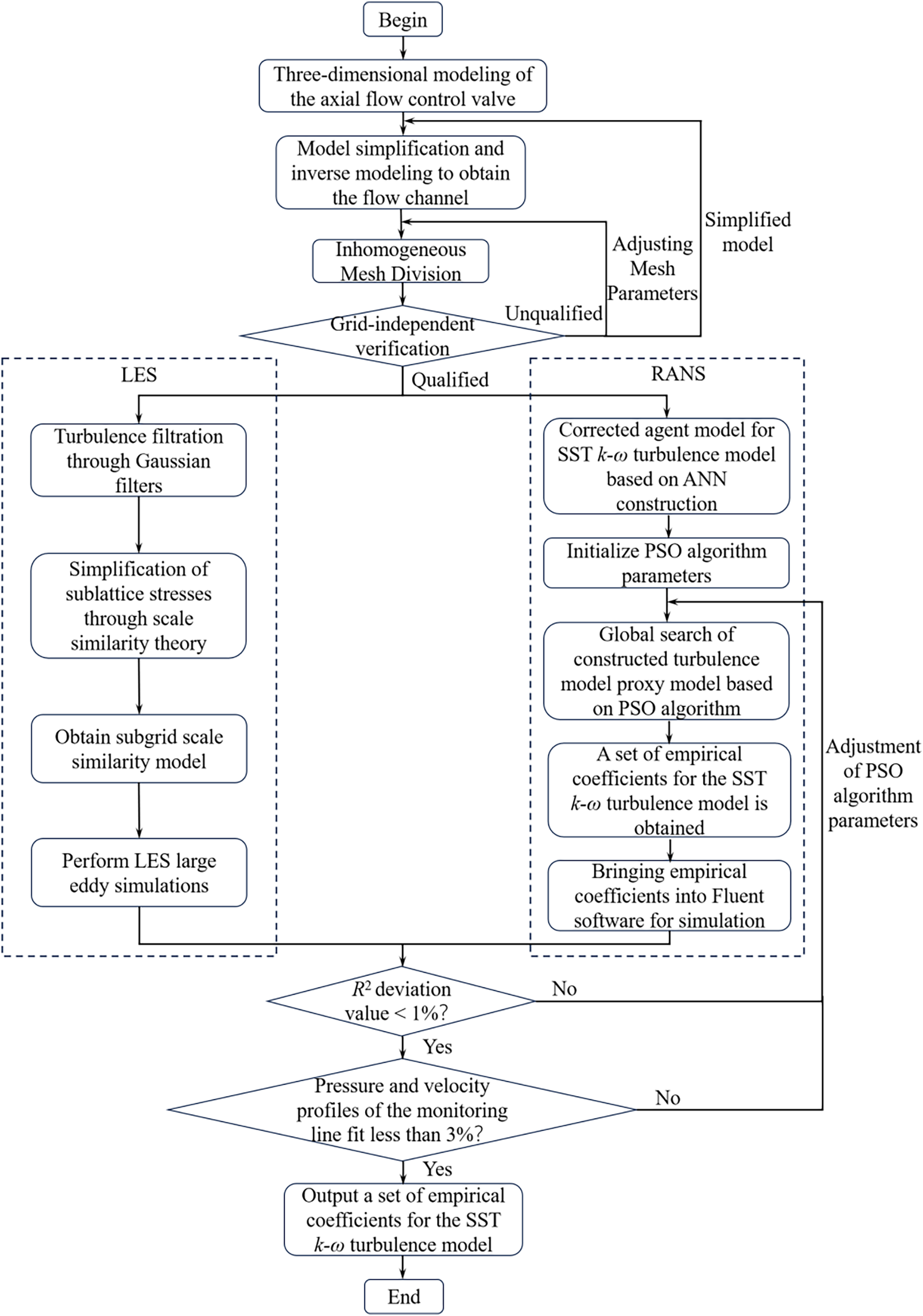
Figure 10: Turbulence model correction flow chart

4.2 Latin Hypercube Sampling-Based Analysis and Dimensionality Reduction of Turbulence Model Parameters

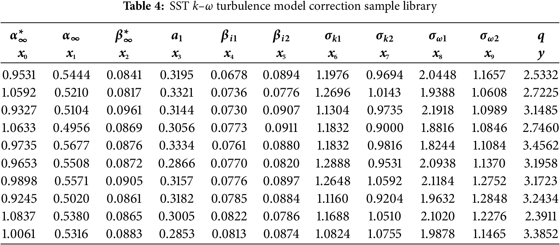
When constructing the surrogate model of the SST k–ω turbulence model objective function of the axial flow control valve, the design of the experiment (DOE) can ensure that the database of the surrogate model is evenly distributed in the domain of definition and accelerate the calculation speed. A good DOE usually needs to meet two requirements. One is the generated sample points, which can adapt to different statistical assumptions. Another requirement is that the generated sample points can cover the design space from small to large. The optimal Latin hypercube algorithm has become the most popular DOE method because of these two characteristics [21]. After the optimal Latin hypercube sampling, 100 sample points were obtained, and the database was obtained by CFD simulation. The SST k–ω turbulence model correction sample library is shown in Table 4. The first 10 columns are input variables, and the last column is the flow value q predicted by CFD simulation, which is unit kg/s, as the output variable.

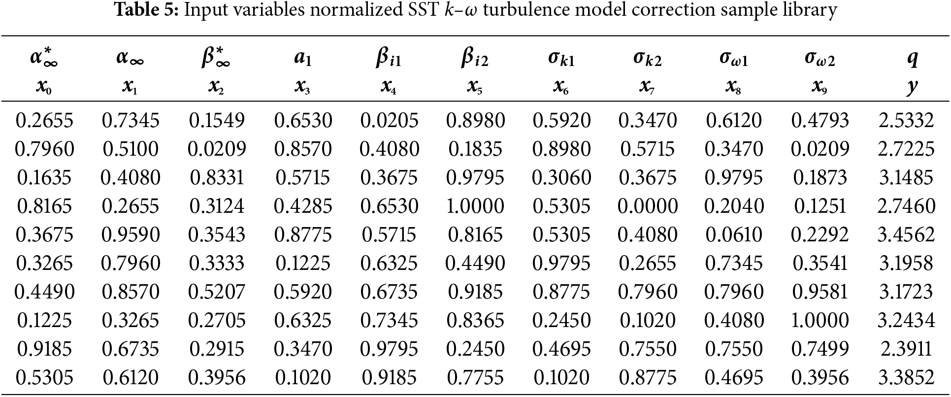
To facilitate the construction of an artificial neural network, the data set is normalized. Normalization can not only reduce the difficulty of data processing but also speed up the solution [22]. When normalizing the data, the data is often mapped to the [0, 1] or [−1, 1] interval. The order of magnitude of the input variables of the sample library is not much different, so it is mapped to the [0, 1] interval according to Formula (3). Since there is only one output variable, the output variables are not normalized.

xi=xi−min(xi)max(xi)−min(xi),i=0,1,2,…,8,9(3)

Among them, xi represents the i-th input variable; min(xi) represents the minimum value of 100 xi after sampling; max(xi) represents the maximum value of 100 xi after sampling.

The sample library after normalization of the input variables is shown in Table 5.

Since the SST k–ω turbulence model has too many coefficient sets, it is necessary to reduce the dimension of the input variables to reduce the number of input variables when constructing the artificial neural network. The significance of the default 10 coefficients of the SST k–ω turbulence model embedded in Fluent software is studied.

Firstly, the significance analysis of the sample library after the normalization of the input variables is carried out. The Pearson correlation coefficient represents the degree of linear correlation between the two variables, which is also called the ‘product-moment correlation coefficient’ or ‘correlation’ for short. For the population, two random variables X and Y are given, denoted by ρX,Y. The calculation formula of the overall correlation coefficient ρX,Y is:

ρX,Y=cov(X,Y)σXσY(4)

here, cov(X, Y) is the covariance of X and Y, σX is the standard deviation of X, and σY is the standard deviation of Y.

When it is used for the sample, it is denoted as the sample correlation coefficient r. Given two random variables X and Y, the calculation formula of the sample correlation coefficient r is:

r=∑i=1n(Xi−X¯)(Yi−Y¯)∑i=1n(Xi−X¯)2∑i=1n(Yi−Y¯)2(5)

Among them, n is the number of samples, Xi and Yi are the i-point observations corresponding to variables X and Y, X¯ is the average of sample X, and Y¯ is the average of sample Y. According to the results of the significance analysis, the relationship between the six most significant variables and the flow value is shown in Fig. 11, and the other parameters are fixed.

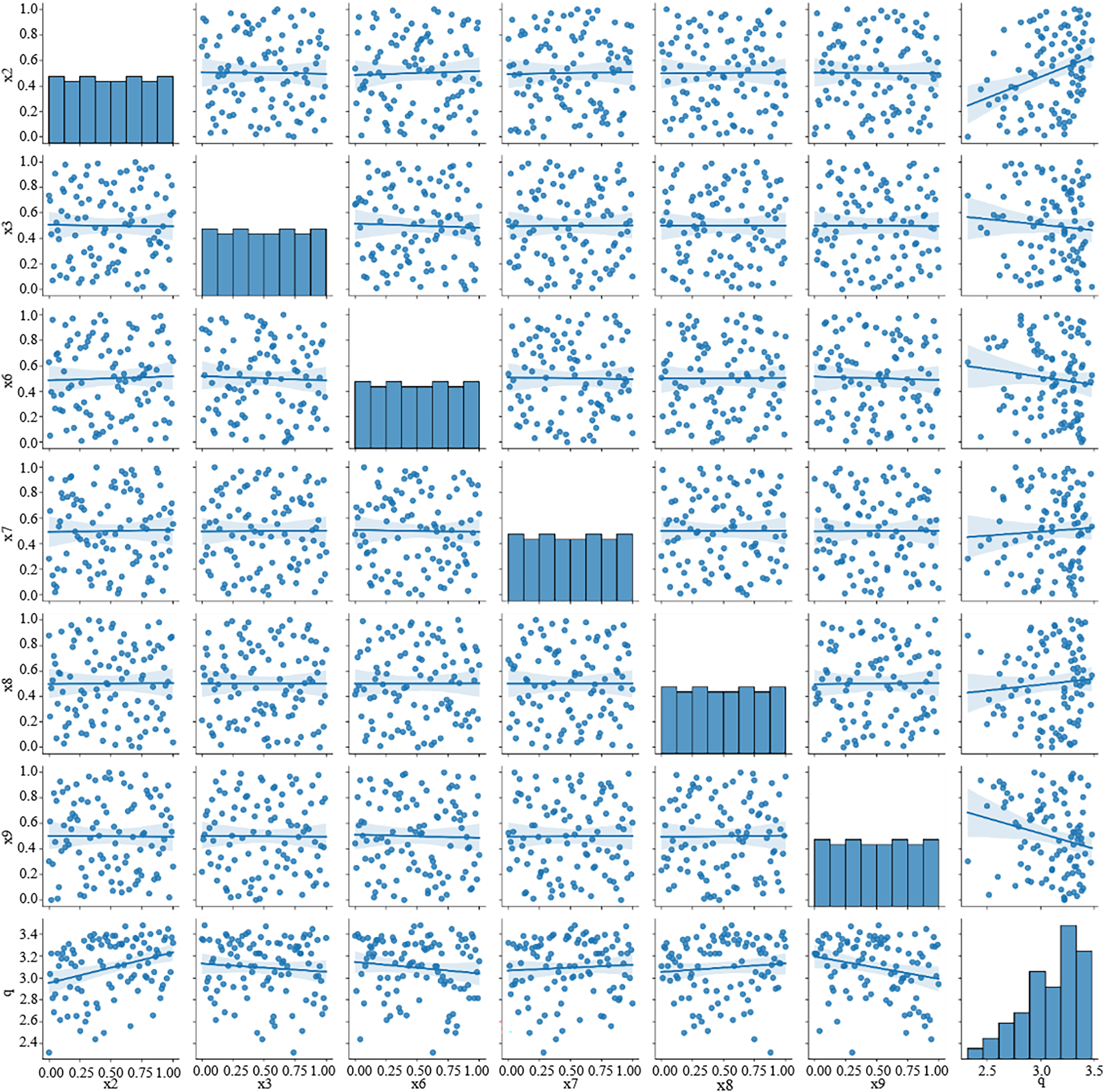
Figure 11: The relationship between significant variables and flow value

According to the results of principal component analysis, it is shown that β∞∗, α1, σk1, σk2, and σω1, σω2 contribute the most to the calculation results. These main coefficients determine the dissipation rate of turbulent kinetic energy, Reynolds stress, diffusion flux of turbulent kinetic energy, and specific dissipation rate. The initial values of the six main coefficients are:

β∞∗=0.09, α1=0.31, σk1=1.176

σk2=1, σω1=2, σω2=1.168

Among them, β∞∗ is the coefficient of the mixing function used for the conversion of the k–ε turbulence model and the k–ω turbulence model, α1 determines the turbulent viscosity, σk1 and σk2 are used to characterize the diffusion flux of turbulent kinetic energy, and σω1 and σω2 represent the turbulent kinetic energy dissipation rate of the diffusion flow.

4.3 Construction of ANN Surrogate Model

Due to the lack of structure of the objective function, there are many difficulties in the SST k–ω turbulence model correction of the axial flow control valve. To save the computational cost, the SST k–ω turbulence model correction problem of the axial flow control valve is considered as a black box optimization problem. For the method of solving the black box problem, the best way is to approximate the black box function by continuously iterating the surrogate model, and then optimizing the black box function (i.e., the objective function). Neural networks are suitable for a large number of general or specific problems. Kolmogorov’s theorem proves that any continuous function of N variables can be approximated by a one-layer artificial feedforward neural network with one hidden layer [23,24]. Therefore, the artificial neural network (ANN) can be used to construct the surrogate model of the SST k–ω turbulence model of the axial flow control valve to correct the black box function.

The ANN is composed of multiple neurons, and the signal is collected from the neurons in the form of weighted input, and the weighted output is forwarded to other neurons by using the activation function. Information transmission may pass through one layer or through multiple layers of neurons. The steps of using the artificial neural network method to construct the SST k–ω turbulence model correction surrogate model of the axial flow control valve are as follows (Fig. 12):

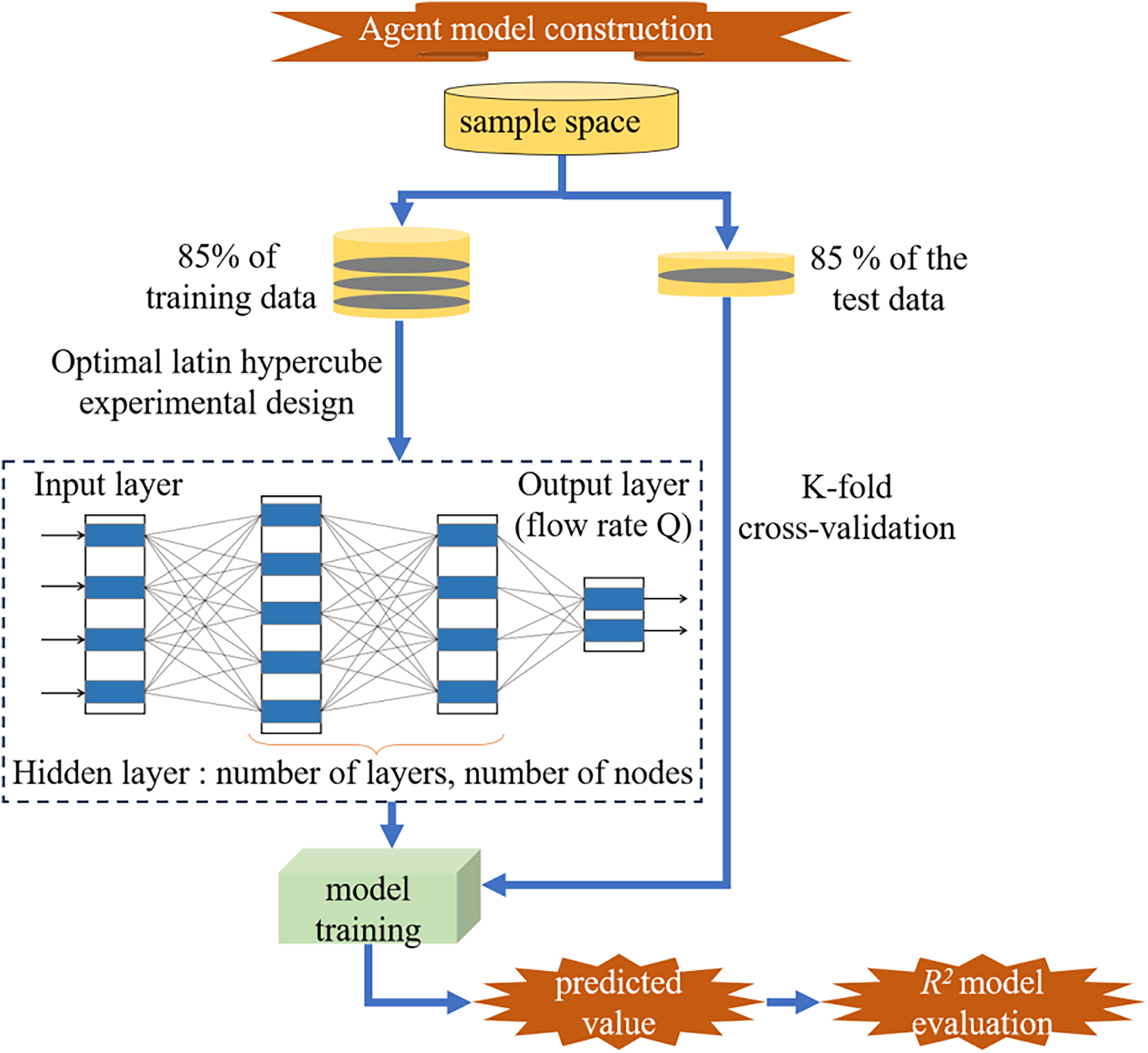
Figure 12: Agent model construction process

When constructing the neural network, it is necessary to select and adjust the value of the solver, the activation function, the regularization function, and the number of hidden layers. According to a large number of previous research results and the comparison in the construction process, it is found that the ‘L-BFGS’ solver (Limited-memory Broyden-Fletcher-Goldfarb-Shanno algorithm) is the most efficient, and the algorithm is an improvement of the Broyden-Fletcher-Goldfarb-Shanno algorithm [25]. The Sigmoid function, also known as the hyperbolic tangent function, is the earliest and most widely used activation function in neural networks. When used as the output function of the hidden layer of the neural network, the Sigmoid function can map a real number between [0, 1]. The number of neurons and regularization parameters of each layer are adjusted in real-time during the construction of the surrogate model. Python 3.9 is used for programming when constructing the ANN turbulence model correction surrogate model.

To minimize the deviation caused by random sampling during training, the k-fold cross-validation algorithm is usually used. A hierarchical 10-fold cross-validation method is used to evaluate the predictive performance of the surrogate model for the output variables.

The correction of SST k–ω turbulence model coefficients of the axial flow control valve is a typical regression prediction problem. Therefore, to better measure the performance of the regression prediction surrogate model, R-Square, that is, R2, is used to evaluate the performance of the model. The closer the R2 value is to 1, the closer the value of the prediction variable is to the experimental value of the variable obtained by the CFD simulation experiment in the validation set [26]. The value of R2 can be calculated by Formula (6).

R2(y,y^)=1−∑i=1n(yi−y^i)2∑i=1n(yi−y¯i)2(6)

Among them, yi represents the experimental value of the variable obtained by the CFD simulation experiment, y¯i represents the average value of the experimental value of the variable, and y^i represents the predicted value of the surrogate model.

R2 is used to evaluate the artificial neural network surrogate model of the SST k–ω turbulence model coefficient of the axial flow control valve. The model evaluation result is R2 = 0.9745, and the model evaluation result is shown in Fig. 13.

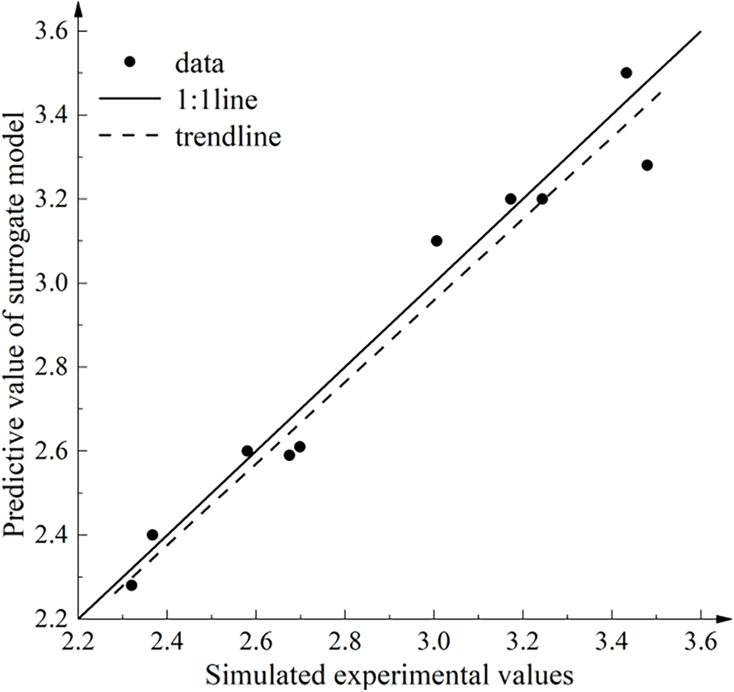
Figure 13: Turbulence model modified ANN surrogate model R2 model evaluation results

From the evaluation results of the ANN surrogate model R2 model in Fig. 13, it can be seen that the trend lines of the 10 verification points are below the 1:1 line and parallel to the 1:1 line.

The approximate function image of the turbulence model constructed by an artificial neural network is shown in Fig. 14.

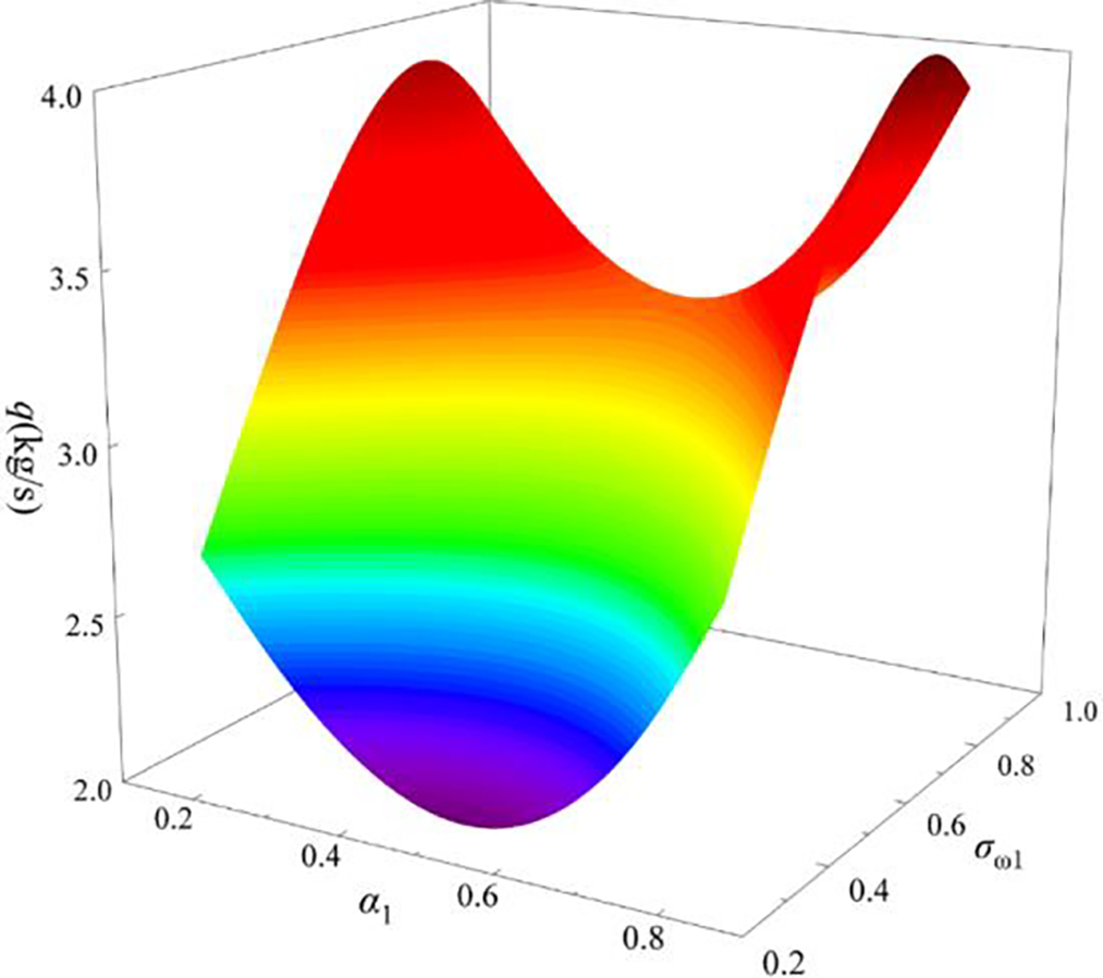
Figure 14: Image of surrogate model constructed by artificial neural network

4.4 PSO Algorithm Global Search

The fundamental principle of the Particle Swarm Optimization (PSO) algorithm involves information exchange among particles within a population to identify optimal solutions. During each iteration, each particle updates its position and velocity by tracking two optimal values: the personal best (Pbest) and the global best (gbest). Upon identifying these two optima, the particle adjusts its trajectory using Eq. (7) to update its velocity and position.

{vidk+1=wvidk+c1r1(pbestidk−xidk)+c2r2(gbestidk−xidk)xidk+1=xidk+vidk+1(7)

In Eq. (7), i = 1, 2, ∙∙∙, n; d = 1, 2, ∙∙∙, n; k represents the iteration number of particles; c1 is the cognitive learning factor and c2 is the social learning factor, typically set as c1 = c2 = 2; r1 and r2 are random coefficients uniformly distributed in the interval [0, 1]; w denotes the inertia weight, where a larger w value indicates stronger global exploration capability while a smaller w enhances local exploitation, w employs a linear decreasing strategy. The PSO algorithm exhibits gradient-free characteristics and demonstrates efficient parallel computing capabilities. Its swarm intelligence mechanism effectively avoids the drawbacks of traditional manual parameter tuning while requiring fewer adjustable parameters compared to genetic algorithms.

PSO particle swarm optimization algorithm is a commonly used global search algorithm. Particle swarm optimization determines the best position for each particle and evaluates the function value of each particle to finally achieve the best [27,28]. The PSO particle swarm optimization algorithm is used to search the turbulence model modified ANN surrogate model. The search process is shown in Fig. 15:

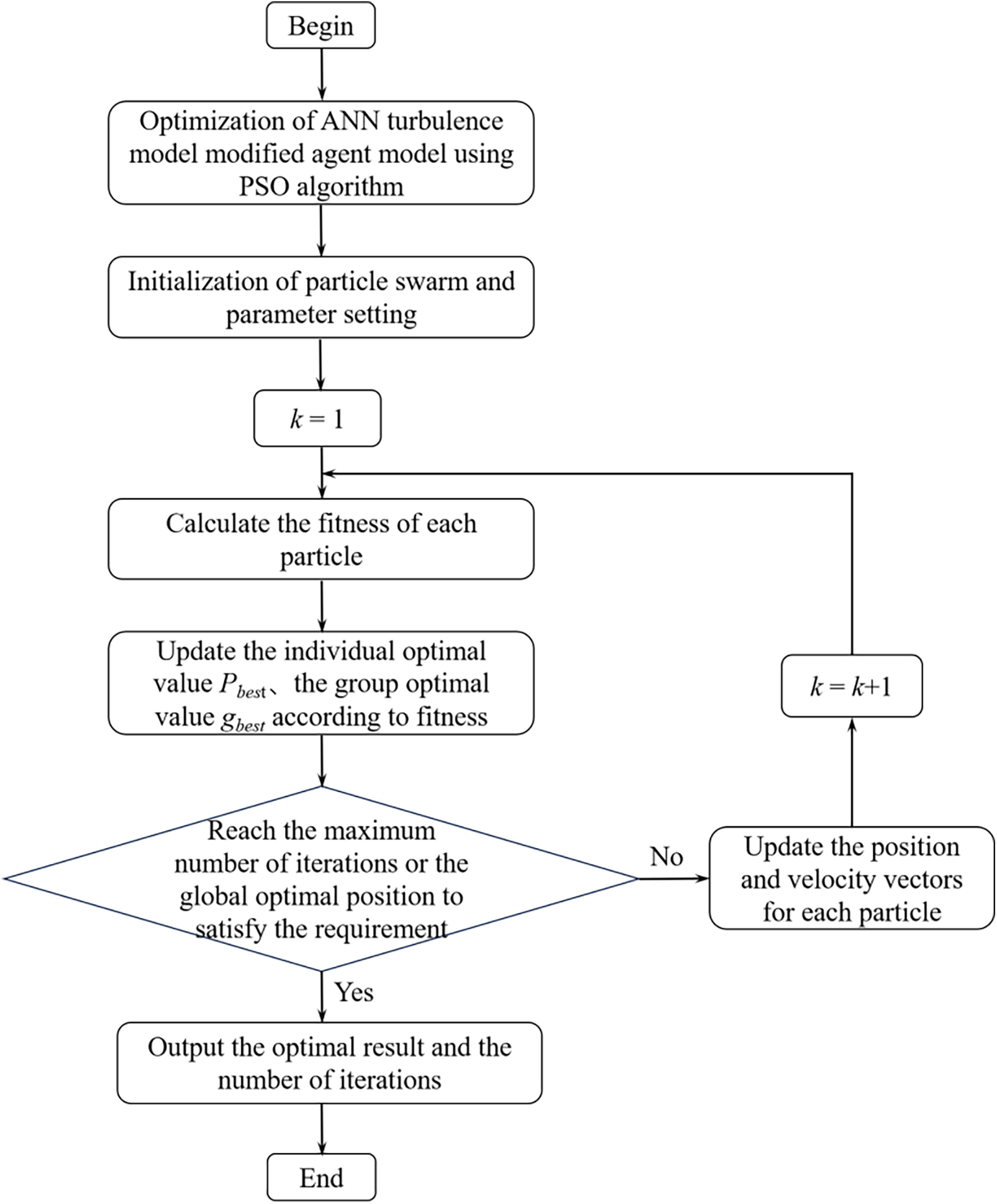
Figure 15: Flow chart of PSO algorithm searching turbulence model to modify ANN surrogate model

The PSO particle swarm optimization algorithm is used to search the turbulence model modified ANN surrogate model. Firstly, a batch of initial solutions is generated, and the initial velocity of the particles is given. The initial solution is used as the initial population, and the fitness (objective function value) of each solution in the initial population is calculated. The individual optimal solution Pbest and the group optimal solution gbest are updated, and then the current solution set is updated by using the velocity and position update formula built in the particle swarm optimization algorithm. The fitness (objective function value) of each solution in the current solution set is calculated until the individual optimal solution and the group optimal solution meet the iteration termination condition, and then the optimal solution searched is output. The PSO global search algorithm is used to construct the global search process of the ANN turbulence model correction surrogate model, as shown in Fig. 16.

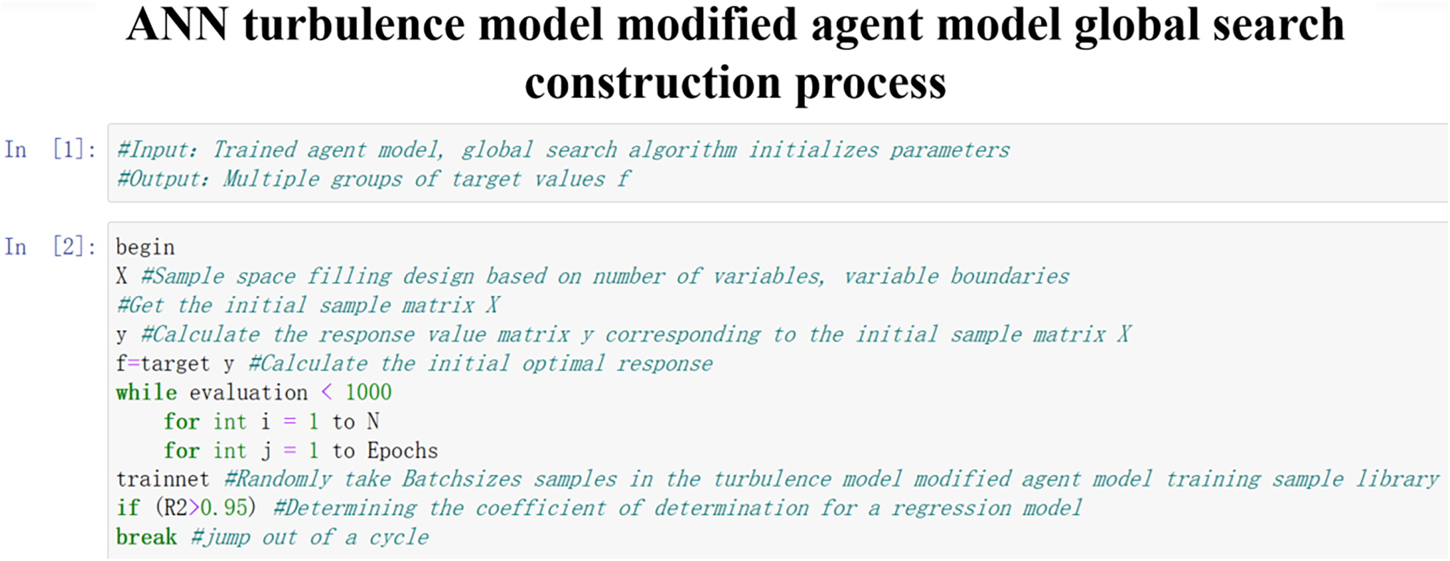
Figure 16: PSO global search process construction ideas

The convergence curve of the global optimization process of the turbulence model correction surrogate model of the axial flow control valve using the PSO algorithm is shown in Fig. 17.

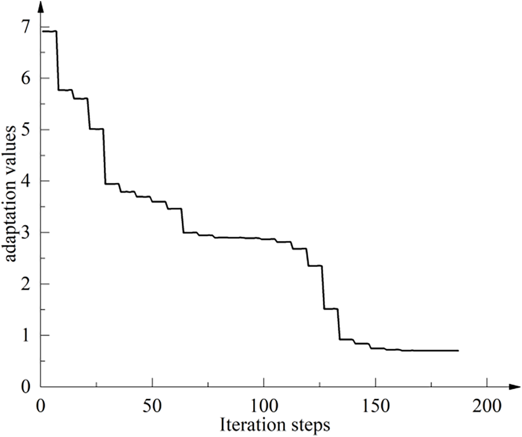
Figure 17: Convergence curve of PSO optimization algorithm

The PSO algorithm is used to globally search the ANN turbulence model modified surrogate model, and the empirical coefficients of five groups of predicted flow values close to the LES large eddy simulation results are obtained.

β∞∗=0.125,a1=1.64,σk1=1.86,σk2=0.065,σω1=1.3,σω2=0.05β∞∗=0.116,a1=1.86,σk1=1.92,σk2=0.062,σω1=1.24,σω2=0.04β∞∗=0.122,a1=1.39,σk1=1.99,σk2=0.058,σω1=1.2,σω2=0.03β∞∗=0.13,a1=1.74,σk1=1.95,σk2=0.047,σω1=1.18,σω2=0.06β∞∗=0.142,a1=1.68,σk1=1.78,σk2=0.073,σω1=1.46,σω2=0.02

After the five sets of data were imported into Fluent for simulation calculation and compared with the LES large eddy simulation results, the empirical coefficient of the modified SST k–ω turbulence model was determined as follows:

β∞∗=0.122,a1=1.39,σk1=1.99,σk2=0.058,σω1=1.2,σω2=0.03

5  Analysis of Simulation Results after Empirical Coefficient Correction

The SST k–ω turbulence model with the modified empirical coefficient is used to simulate the internal flow of the axial flow control valve under the test conditions and compared with the LES large eddy simulation results before the correction.

5.1 The Corrected Flow Characteristic Curve

After modifying the turbulence model, the flow coefficient Kv of the axial flow control valve is calculated according to Formula (1), and the calculation results are shown in Table 6.

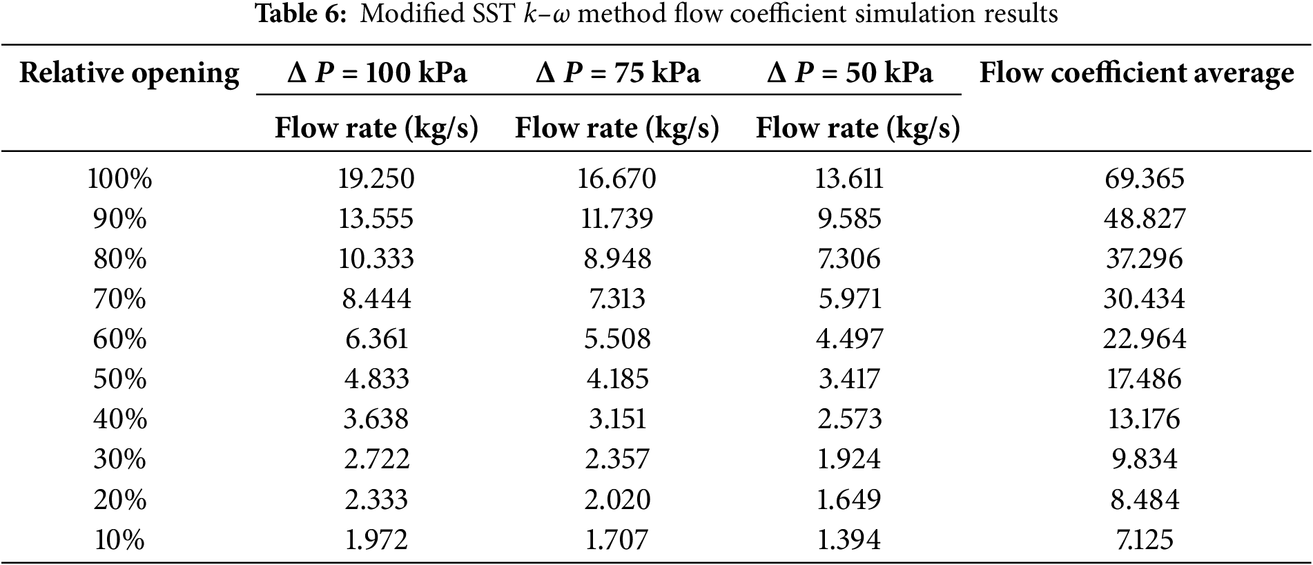
According to the calculation results of Table 6, the flow characteristic curve of the axial flow control valve is drawn. The comparison between the flow characteristic curve before and after the correction and the LES large eddy simulation is shown in Fig. 18.

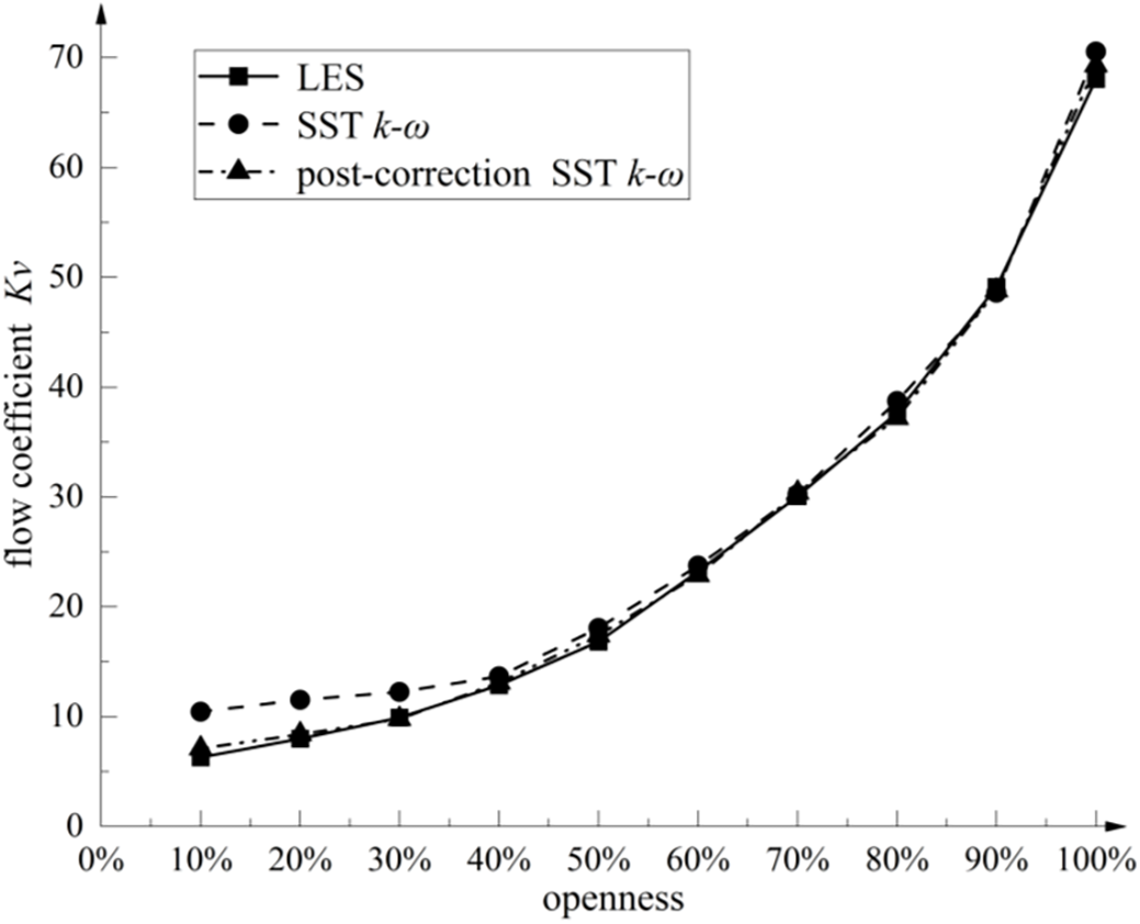
Figure 18: Flow characteristics of the axial flow control valve before and after turbulence model correction

It can be seen from Fig. 18 that the deviation between the predicted value of the internal flow of the axial flow control valve by the modified SST k–ω turbulence model and the predicted value of the LES large eddy simulation is much smaller than that before the correction, which shows the effectiveness of the correction method.

5.2 The Corrected Internal Flow Field

From Fig. 18, it can be seen that the SST k–ω simulation accuracy is significantly improved at a small opening, which is equivalent to the LES large eddy simulation level. The simulation accuracy of SST k–ω under a large opening is also improved, and the flow condition at 100% opening is selected for analysis. The simulation results on the horizontal section inside the 100% opening of the axial flow control valve with the modified turbulence model are shown in Figs. 19 and 20.

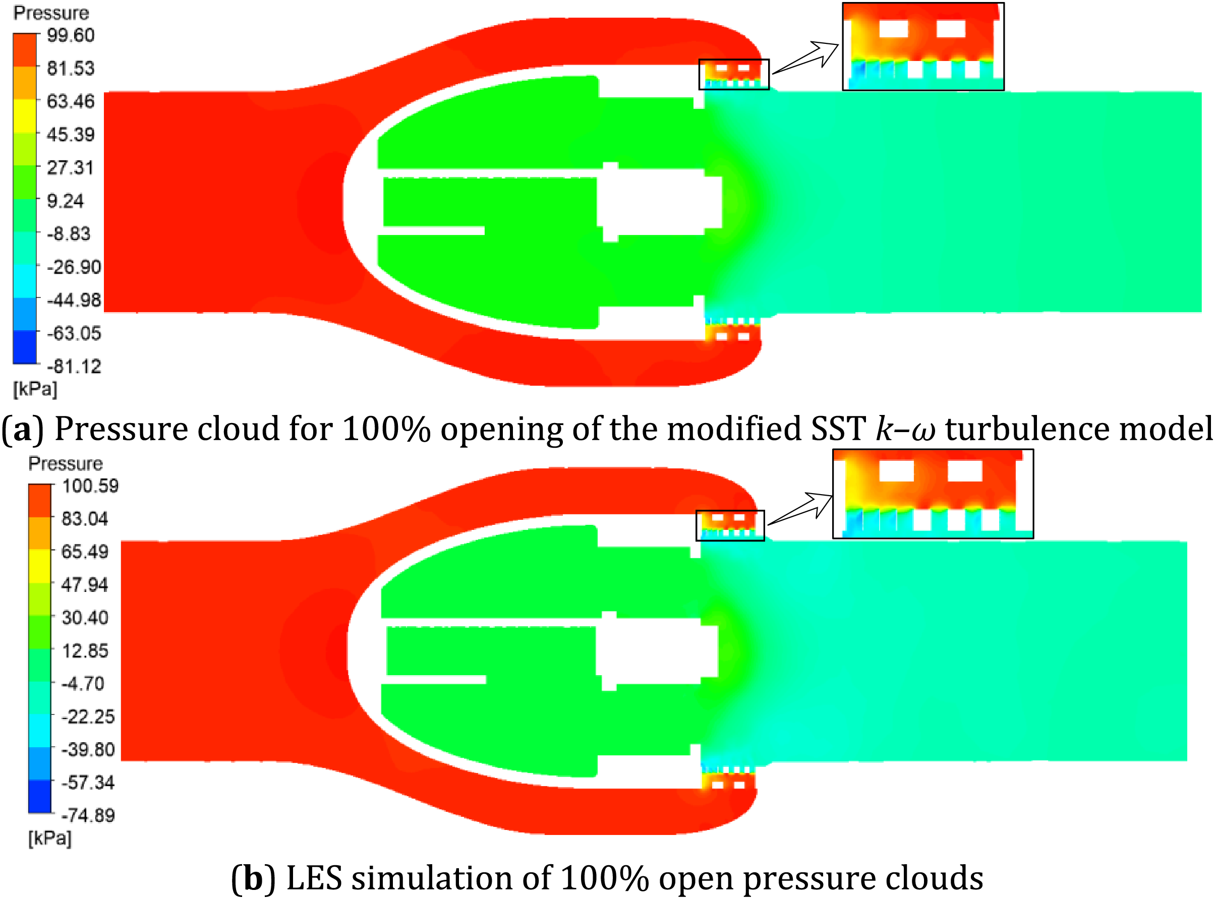
Figure 19: Comparison of corrected SST k–ω simulation and LES simulation pressure clouds at 100% opening

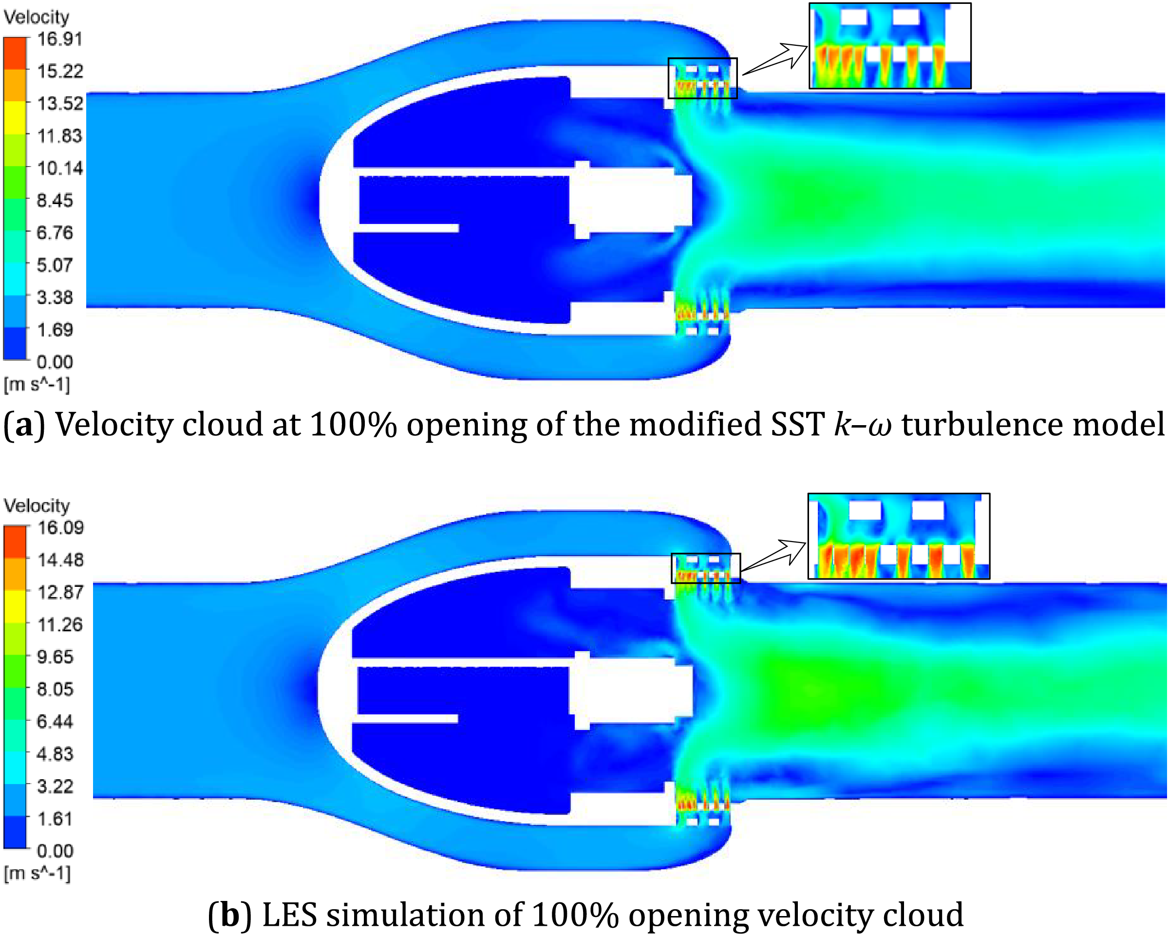
Figure 20: Velocity cloud comparison between modified SST k–ω simulation and LES simulation at 100% openness

The pressure distribution at 100% opening of the axial flow control valve simulated by the modified SST k–ω turbulence model is shown in Fig. 19a: the flow passage through the multi-stage pressure-reducing assembly exhibits a more physically realistic pressure gradient distribution in the modified SST k–ω simulation, showing significantly improved continuity compared to the pre-modification results, and the extreme value of the upper and lower limits of the pressure is compared with the LES large eddy simulation results in Fig. 19b. The consistency of the value and the change trend is greatly improved before the correction. The global minimum pressure under the test condition is −81.12 kPa, which is about 7.6% different from the LES large eddy simulation results and 61.4% different before correction. The global maximum pressure under the test condition is 99.6 kPa, which is about 1.1% different from the LES large eddy simulation results.

The velocity distribution cloud diagram at 100% opening of the axial flow control valve simulated by the modified SST k–ω turbulence model is shown in Fig. 20a: the modified SST k–ω turbulence model has enhanced diffusion of turbulent kinetic energy, the jet width is closer to the LES results, and the predictions of the recirculation zone are closer to the LES results, and the velocity decay trends of fluid velocity is highly consistent with the LES large eddy simulation results in Fig. 20b. The global maximum velocity under the test condition is 16.91 m/s, which is about 4.8% different from the LES large eddy simulation results and 30.2% different before correction.

From the comparative analysis of the pressure cloud map and the velocity cloud map, it can be seen that the modified SST k–ω turbulence model’s ability to capture the internal flow information of the axial flow control valve is close to the LES large eddy simulation.

The simulation results of four depressurization routes at the multi-stage depressurization of the horizontal section of the axial flow control valve SST k–ω and LES are monitored. Taking the simulation results of the SST k–ω method as an example, the midline of the distance between the two-stage pressure-reducing sleeves is taken as the origin, and the fluid flow direction is taken as the positive direction. The schematic diagram of the pressure and velocity change monitoring line position of the four depressurization routes of the SST k–ω and LES simulation methods is shown in Fig. 21. The center section of the two-stage step-down sleeve is at the zero point of the coordinate. The spacing between the two-stage step-down sleeves is 4 mm, and the thickness of the two-stage sleeves is 3 mm. The outer side of the first-stage sleeve is between −15 and −5 of the coordinate axis.

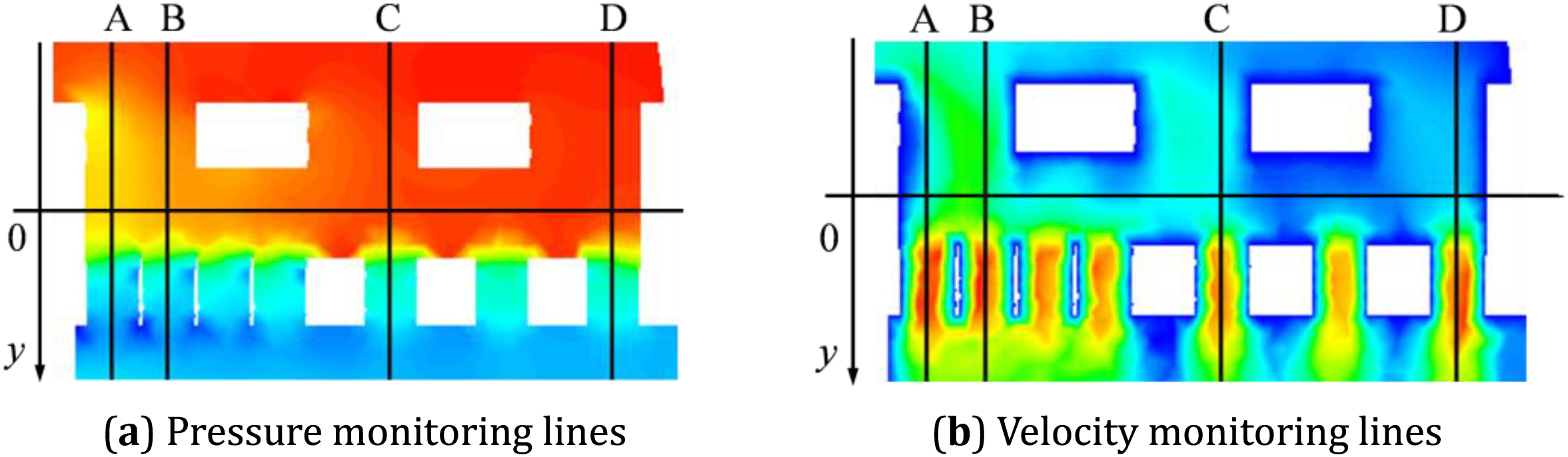
Figure 21: Schematic diagram of monitoring line location at 100% openness

Using the monitoring method shown in Fig. 21, the pressure and velocity changes at the multi-stage pressure drop of the axial flow control valve after the modified turbulence model are compared with the LES large eddy simulation results, as shown in Figs. 22 and 23.

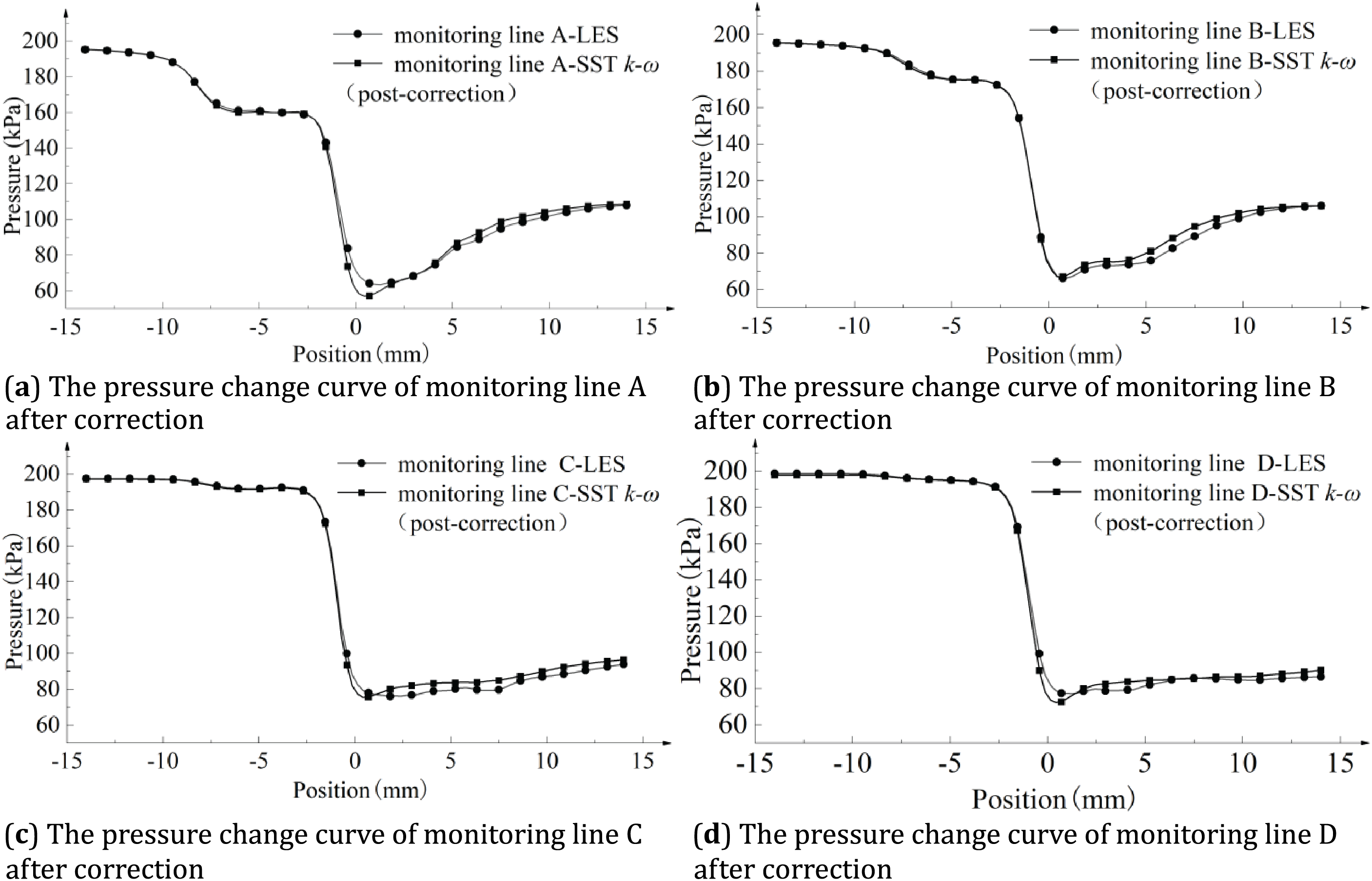
Figure 22: Comparison of corrected SST k–ω simulation and large eddy simulation pressure monitoring results at 100% opening

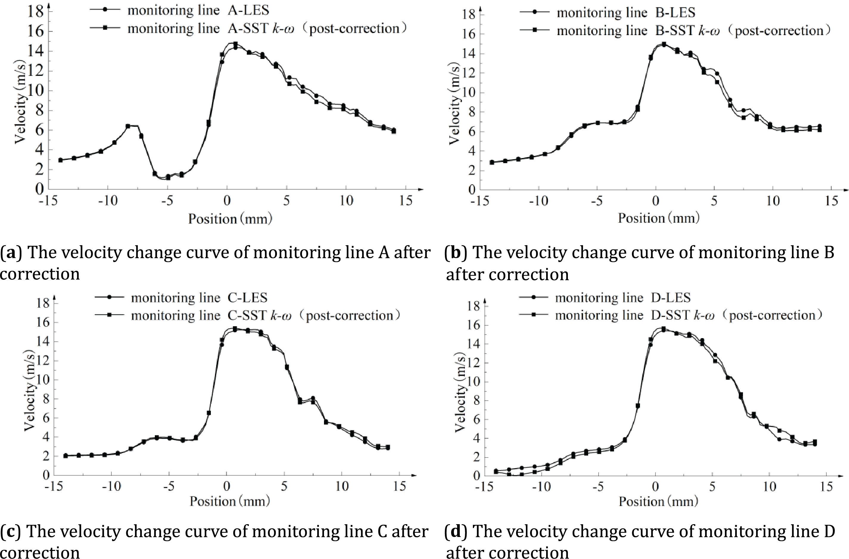
Figure 23: Comparison of SST k–ω simulation and large eddy simulation velocity monitoring results at 100% opening after correction

Fig. 22 shows the pressure changes of the modified SST k–ω simulation and LES large eddy simulation at the typical position of the multi-stage pressure-reducing sleeve. The prediction of the internal flow information of the axial flow control valve by the modified SST k–ω turbulence model is very close to the prediction results of the LES large eddy simulation, whether it is the pressure change trend or the pressure fluctuation after the violent flow.

Fig. 23 shows the velocity changes of the modified SST k–ω simulation and LES large eddy simulation at the typical position of the multi-stage step-down sleeve. Whether the velocity change trend or the velocity change after the violent flow, the prediction of the modified SST k–ω turbulence model is very close to the prediction results of the LES large eddy simulation.

In summary, the SST k–ω turbulence model after correcting the empirical coefficient has greatly improved the capture accuracy of the internal flow information of the axial flow control valve, which is close to the simulation accuracy of LES large eddy simulation.

5.3 Computational Efficiency Analysis

The work in this paper was done with a workstation configured with Intel Core i9-14900K (24 cores, 32 threads, 3.2 GHz), 128 GB RAM, and the computational costs of all three methods (original SST k–ω, modified SST k–ω, and LES) were evaluated using the same hardware and grid configuration. For the typical case of 100% openness, the original SST k–ω required 4.2 h, the modified SST k–ω (post-calibration) required 4.5 h due to additional iterations, and LES required 48 h. The modified SST k–ω model reduces the deviation from the LES results to within 3% while maintaining computational efficiency. Although the calibration process introduced a marginal increase in runtime, it is still an order of magnitude faster than LES, which requires 10 times the resources. This makes the calibration model suitable for industrial applications where both accuracy and cost are critical.

6  Conclusion

To enhance the predictive accuracy of the SST k–ω turbulence model for internal flows in axial control valves, this study develops an artificial neural network (ANN) surrogate model. The model takes the SST k–ω empirical coefficients as inputs and predicts the corresponding flow capacity. Subsequently, a particle swarm optimization (PSO) algorithm globally optimizes these empirical coefficients, enabling the numerical simulations to more closely match real-world valve performance at a reduced computational cost. Key findings are summarized as follows:

(1)   The SST k–ω model demonstrates good agreement with LES results for axial flow control valve openings above 50%. However, as the valve opening decreases below 50%, the SST k–ω simulations begin to diverge from LES predictions, with the deviation becoming more pronounced at smaller openings. This suggests that the SST k–ω model’s accuracy diminishes when simulating the valve’s small-opening conditions.

(2)   The modified SST k–ω turbulence model’s predictions of axial control valve flow characteristics show remarkable consistency with LES data, with deviations constrained to within 3%. These results demonstrate substantial enhancement in the model’s capability to accurately resolve internal flow dynamics.

Although the modified SST k–ω model significantly improves the prediction accuracy of axial flow control valves, it still suffers from the following limitations for small opening conditions (e.g., 10% valve opening). At low openings, the strong flow separation and recirculation zones near the multi-stage sleeves may not be fully resolved by the RANS model, leading to deviations from the LES results. Secondly the empirical coefficients of the modified SST k–ω model, although globally optimized, may require local adjustment for extreme throttling conditions. While LES is more accurate at small openings, its computational cost is too high, and the modified SST k–ω model is more suitable for engineering applications. Subsequent research will investigate adaptive coefficient optimization methodologies for small-opening scenarios to improve computational prediction fidelity.

Acknowledgement: We thank the other members of the Machinery Industry Pump and Special Valve Engineering Research Center, Lanzhou University of Technology team for their support of this study.

Funding Statement: The research was funded by Gansu Provincial Department of Education (Industrial Support Plan Project: 2025CYZC-048).

Author Contributions: The authors confirm contribution to the paper as follows: writing—review & editing, methodology, funding acquisition, supervision: Shuxun Li; writing—original draft, methodology, conceptualization, software, investigation, validation: Yuhao Tian; writing—review & editing, software: Guolong Deng, Wei Li; writing—review & editing: Yinggang Hu; writing—review & editing: Xiaoya Wen. All authors reviewed the results and approved the final version of the manuscript.

Availability of Data and Materials: The data that supports the findings of this study are available from the corresponding author upon reasonable request.

Ethics Approval: Not applicable.

Conflicts of Interest: The authors declare no conflicts of interest to report regarding the present study.

References

1. Jin HZ, Tang KM, Liu XF, Wang C. Numerical simulation and experimental study on internal depressurization flow characteristics of a multi-layer sleeve regulating valve. J Appl Fluid Mech. 2023;16(4):877–90. doi:10.47176/jafm.16.04.1571. [Google Scholar] [CrossRef]

2. Lin Z, Ma C, Xu H, Li X, Cui B, Zhu Z. Numerical and experimental studies on hydrodynamic characteristics of sleeve regulating valves. Flow Meas Instrum. 2017;53:279–85. doi:10.1016/j.flowmeasinst.2016.12.001. [Google Scholar] [CrossRef]

3. Li S, Deng G, Hu Y, Yu M, Ma T. Optimization of structural parameters of pilot-operated control valve based on CFD and orthogonal method. Results Eng. 2024;21(11):101914. doi:10.1016/j.rineng.2024.101914. [Google Scholar] [CrossRef]

4. Wu S, Liu H, Chen Y. Comparative analysis of regulating characteristics between air-ring flow regulating valve and center butterfly valve. PLoS One. 2021;16(5):e0251943. doi:10.1371/journal.pone.0251943. [Google Scholar] [PubMed] [CrossRef]

5. Tao J, Lin Z, Ma C, Ye J, Zhu Z, Li Y, et al. An experimental and numerical study of regulating performance and flow loss in a V-port ball valve. J Fluids Eng. 2020;142(2):021207. doi:10.1115/1.4044986. [Google Scholar] [CrossRef]

6. Singh D, Aliyu AM, Charlton M, Mishra R, Asim T, Oliveira AC. Local multiphase flow characteristics of a severe-service control valve. J Petrol Sci Eng. 2020;195(10):107557. doi:10.1016/j.petrol.2020.107557. [Google Scholar] [CrossRef]

7. Guo G, Zhang R, Yu H. Evaluation of different turbulence models on simulation of gas-liquid transient flow in a liquid-ring vacuum pump. Vacuum. 2020;180(5):109586. doi:10.1016/j.vacuum.2020.109586. [Google Scholar] [CrossRef]

8. Tiselj I, Flageul C, Oder J. Direct numerical simulation and wall-resolved large eddy simulation in nuclear thermal hydraulics. Nucl Technol. 2020;206(2):164–78. doi:10.1080/00295450.2019.1614381. [Google Scholar] [CrossRef]

9. Raje P, Sinha K. Anisotropic SST turbulence model for shock-boundary layer interaction. Comput Fluids. 2021;228(7):105072. doi:10.1016/j.compfluid.2021.105072. [Google Scholar] [CrossRef]

10. Menter F, Hüppe A, Matyushenko A, Kolmogorov D. An overview of hybrid RANS-LES models developed for industrial CFD. Appl Sci. 2021;11(6):2459. doi:10.3390/app11062459. [Google Scholar] [CrossRef]

11. Abdolrasol MGM, Suhail Hussain SM, Ustun TS, Sarker MR, Hannan MA, Mohamed R, et al. Artificial neural networks based optimization techniques: a review. Electronics. 2021;10(21):2689. doi:10.3390/electronics10212689. [Google Scholar] [CrossRef]

12. Gad AG. Particle swarm optimization algorithm and its applications: a systematic review. Arch Comput Meth Eng. 2022;29(5):2531–61. doi:10.1007/s11831-021-09694-4. [Google Scholar] [CrossRef]

13. Zhang Y, He C, Sun L. Optimization of an ejector to mitigate cavitation phenomena with coupled CFD/BP neural network and particle swarm optimization algorithm. Prog Nucl Energy. 2022;153:104412. doi:10.1016/j.pnucene.2022.104412. [Google Scholar] [CrossRef]

14. Qidwai MO, Badruddin IA, Khan NZ, Khan MA, Alshahrani S. Optimization of microjet location using surrogate model coupled with particle swarm optimization algorithm. Mathematics. 2021;9(17):2167. doi:10.3390/math9172167. [Google Scholar] [CrossRef]

15. Babanezhad M, Behroyan I, Nakhjiri AT, Marjani A, Rezakazemi M, Heydarinasab A, et al. Investigation on performance of particle swarm optimization (PSO) algorithm based fuzzy inference system (PSOFIS) in a combination of CFD modeling for prediction of fluid flow. Sci Rep. 2021;11(1):1505. doi:10.1038/s41598-021-81111-z. [Google Scholar] [PubMed] [CrossRef]

16. Li Z, Hoagg JB, Martin A, Bailey SCC. Retrospective cost adaptive Reynolds-averaged Navier-Stokes k–ω model for data-driven unsteady turbulent simulations. J Comput Phys. 2018;357(1):353–74. doi:10.1016/j.jcp.2017.11.037. [Google Scholar] [CrossRef]

17. Holgate J, Skillen A, Craft T, Revell A. A review of embedded large eddy simulation for internal flows. Arch Comput Methods Eng. 2019;26(4):865–82. doi:10.1007/s11831-018-9272-5. [Google Scholar] [CrossRef]

18. Kaak ARS, Çelebioğlu K, Bozkuş Z, Ulucak O, Aylı E. A novel CFD-ANN approach for plunger valve optimization: cost-effective performance enhancement. Flow Meas Instrum. 2024;97(1):102589. doi:10.1016/j.flowmeasinst.2024.102589. [Google Scholar] [CrossRef]

19. Langtry RB, Menter FR. Correlation-based transition modeling for unstructured parallelized computational fluid dynamics codes. AIAA J. 2009;47(12):2894–906. doi:10.2514/1.42362. [Google Scholar] [CrossRef]

20. Zeng F, Zhang W, Li J, Zhang T, Yan C. Adaptive model refinement approach for Bayesian uncertainty quantification in turbulence model. AIAA J. 2022;60(6):3502–16. doi:10.2514/1.j060889. [Google Scholar] [CrossRef]

21. Wei W, Tao T, Si L, Wang G, Yan Q. Design and optimization of bionic Nautilus volute for a hydrodynamic retarder. Eng Appl Comput Fluid Mech. 2023;17(1):2273391. doi:10.1080/19942060.2023.2273391. [Google Scholar] [CrossRef]

22. Pan C, Lv Z, Hua X, Li H. The algorithm and structure for digital normalized cross-correlation by using first-order moment. Sensors. 2020;20(5):1353. doi:10.3390/s20051353. [Google Scholar] [PubMed] [CrossRef]

23. Abidoye LK, Mahdi FM, Idris MO, Alabi OO, Wahab AA. ANN-derived equation and ITS application in the prediction of dielectric properties of pure and impure CO2. J Clean Prod. 2018;175(3):123–32. doi:10.1016/j.jclepro.2017.12.013. [Google Scholar] [CrossRef]

24. Ozoegwu CG. Artificial neural network forecast of monthly mean daily global solar radiation of selected locations based on time series and month number. J Clean Prod. 2019;216:1–13. doi:10.1016/j.jclepro.2019.01.096. [Google Scholar] [CrossRef]

25. Alpak F, Gao G, Florez H, Shi S, Vink J, Blom C, et al. A machine-learning-accelerated distributed LBFGS method for field development optimization: algorithm, validation, and applications. Comput Geosci. 2023;27(3):425–50. doi:10.1007/s10596-023-10197-3. [Google Scholar] [CrossRef]

26. Xu X, Du H, Lian Z. Discussion on regression analysis with small determination coefficient in human-environment researches. Indoor Air. 2022;32(10):e13117. doi:10.1111/ina.13117. [Google Scholar] [PubMed] [CrossRef]

27. Piotrowski AP, Napiorkowski JJ, Piotrowska AE. Particle swarm optimization or differential evolution—a comparison. Eng Appl Artif Intell. 2023;121(11):106008. doi:10.1016/j.engappai.2023.106008. [Google Scholar] [CrossRef]

28. Zheng Q, Feng BW, Liu ZY, Chang HC. Application of improved particle swarm optimisation algorithm in hull form optimisation. J Mar Sci Eng. 2021;9(9):955. doi:10.3390/jmse9090955. [Google Scholar] [CrossRef]