Robot Zero-Moment Control Algorithm Based on Parameter Identification of Low-Speed Dynamic Balance

1  Introduction

Robot zero-moment control technology requires dynamic models as theoretical support. The dynamic model of the collaborative robot can be obtained by the Lagrangian or the Newton-Euler equation, and the dynamic parameters can be identified by some methods. The parameters to be identified in the model mainly include three categories: kinematic, dynamic and friction parameters. Kinematic parameters involve link length, torsion angle, link bias, etc. These are obtained through kinematics calibration and are known as quantities. The dynamic parameters include the mass of the connecting rod, the first mass moment and the moment of inertia. Friction parameters are determined by the friction model. Dynamic parameters and friction parameters must be identified.

Yang et al. [1] developed a robot control/identification scheme to identify the unknown robot kinematic and dynamic parameters with enhanced convergence rate. Jin et al. [2] proposed a new dynamic parameter identification method for flexible joints. Urrea et al. [3] discussed the design and assessment of different parameter identification methods applied to robot systems, such as least squares, extended Kalman filter, Adaptive Linear Neuron (Adaline) neural networks, Hopfield recurrent neural networks and genetic algorithms. Considering the joint elasticity, a novel dynamic parameter identification method is proposed for general industrial robots only with motor encoders [4]. The proposed method can reasonably resolve the problem of mutual opposition within a single criterion and improve the identification robustness compared with other optimisation criteria [5]. An improved integration method is proposed which increases the sampling period by redefining the update condition; it then expands the applied range of the classical method which is more suitable for the working characteristics of a robot servo controller and reduces the speed quantisation error generated by the encoder [6].

Xiao et al. [7] proposed a collision detection algorithm without external sensors which can detect potential collisions in man-robot interaction. A multi-criteria method, in support of the planning of shared human-robot assembly tasks, is presented [8]. To enable the teaching of industrial robots by hand without any force sensors, Zhang et al. [9] put forward a scheme to minimise the external force estimation error and reduce disturbance in the guiding task by using the virtual mass and virtual friction model. Gaz et al. [10] addressed the problem of extracting a feasible set of dynamic parameters characterising the dynamics of a robot manipulator.

To achieve zero moment control in robot teaching, this paper explores the sensorless method on the basis of joint torque compensation. The torque balance equation was established to realise the zero-moment dragging and teaching function of the lightweight collaborative robot. The robot parameter identification based on the least square method was used to accurately identify the robot torque sensitivity and friction.

Given that the robot joint can approximately satisfy the torque balance equation when it is rotating at a low speed, the joint position and motor current value were collected through experiments in the whole process of low-speed motion, which were used as excitation signals to realise the identification of robot dynamics parameters. Finally, an accurate dynamic compensation model was established to realise zero moment dragging. The proposed method is applied to a self-developed collaborative robot, as shown in Fig. 1, and the reliability of the proposed compensation algorithm is verified. This method does not need a multi-dimensional force sensor, the system is simple, the cost is low, and the teaching is flexible, which develops a new way for all kinds of robot teaching with complicated trajectories.

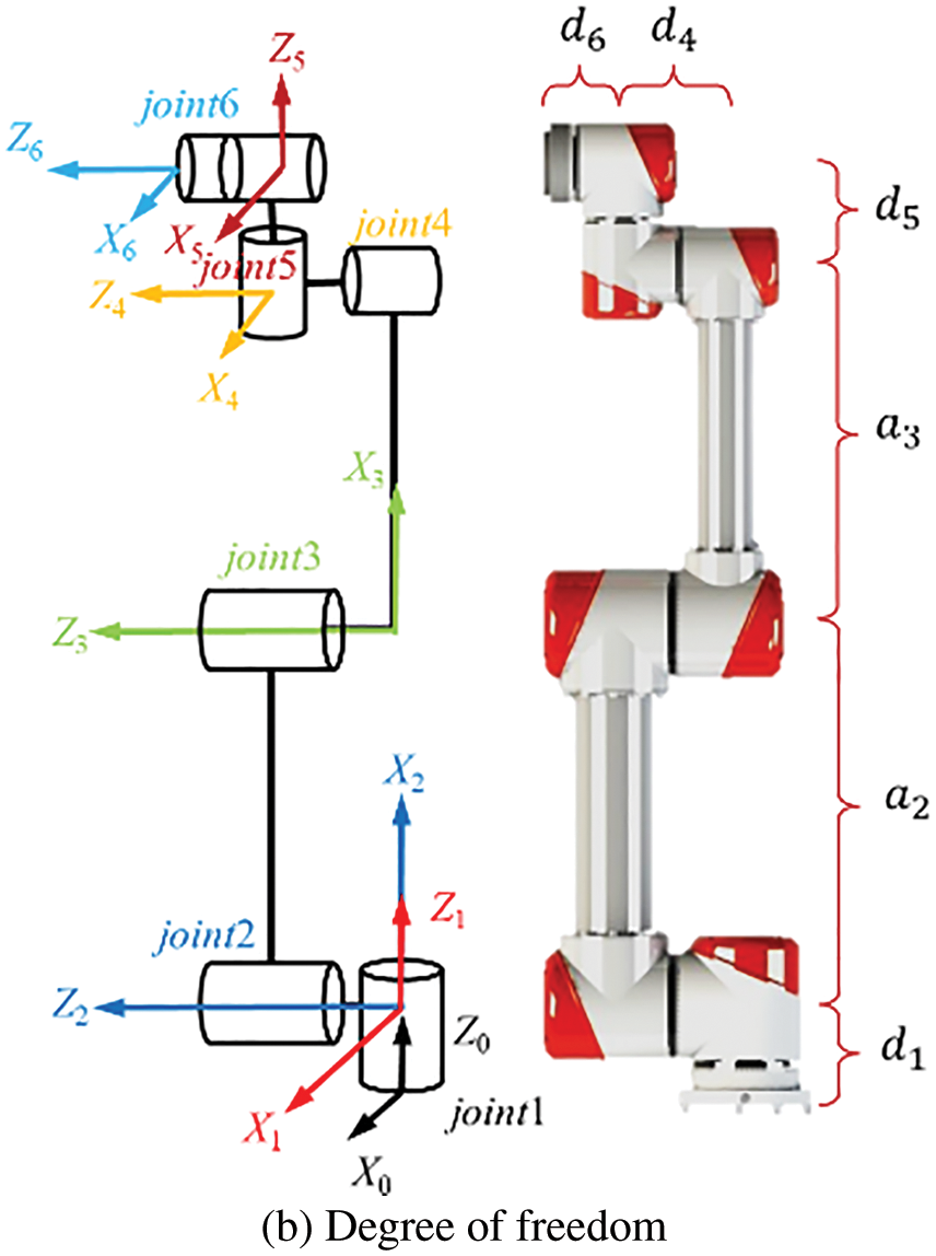
Figure 1: The collaborative robot

2  Zero-Moment Control Based on Torque Compensation

2.1 Zero-Moment Control System

This paper proposes the zero-moment control based on torque compensation. Its essence is that the servo driver works in torque mode and controls the corresponding torque output of each joint motor through the servo driver to overcome the gravity and friction of the robot itself. At this point, the robot must only overcome the small inertial force under the traction of external force to move following the external force.

The entire control system is shown in Fig. 2. Km is the torque constant of the servo controller, G(q) is the gravitational torque of each joint, τf is the friction torque of each joint, τtot direct output torque instruction of the robot controller. The zero-moment control system is a torque control system, its joint position and speed are not controlled, which is convenient for teaching operations.

Figure 2: Zero-moment control system based on torque compensation

Zero-moment control technology based on torque compensation only needs the robot controller to output torque instruction τtot. The torque instruction was mainly used to overcome the gravity and friction caused by the mechanical structure of the robot itself. The process is as follows:

τtot=G(q)+τf.(1)

To meet the requirements of the zero-moment control technology based on torque compensation, the robot control system must have the following functions:

1. Current detection modules must be designed for the drivers of each joint of the robot. The motor drivers of each joint are designed at the end of the motor to facilitate wiring and achieve a compact design, as shown in Fig. 3a. A current detection module based on Hall current sensor was added to the driver, as shown in Fig. 3b.

Figure 3: Current detection system in motor drive

2. In dragging the robot, the robot operator drags the machine to any position and then releases it. The robot can stay in this position without being affected by gravity and friction.

2.2 The Advantages and Disadvantages of the Zero-Moment Control Technology

The zero-moment control technology based on torque control can provide a solution without external sensors. This method can realize flexible operation using a simple algorithm for the direct teaching of lightweight robots. This method has the following advantages and disadvantages [11]:

1. The zero-moment control based on torque mainly realizes the robot joint rotation by controlling the torque/current. Its joint position and speed are not controlled, which is convenient for teaching operation, but the system stability is not as good as the traditional zero-moment control system based on position control.

2. In the zero-moment teaching process, the robot motion is driven directly by the force of the operator, which has better flexibility and accuracy than the traditional zero-moment control system based on position.

3. Zero-moment control system based on torque does not need any sensor, such as a six-dimensional force sensor, or joint torque sensor, so the cost is low.

4. The calculation of the zero-moment control system based on torque is less than that based on position.

5. In the zero-moment control system based on torque, the inertia force of the robot must be overcome by the operator. Therefore, the algorithm is not suitable for robots with large dead-weight.

3  Torque Sensitivity and Static Friction Parameter Identification

The zero-moment dragging and teaching function of the lightweight collaborative robot based on joint shaft torque balance control was not dependent on the external additional torque sensor. When the robot was in a state of dragging and teaching mode, the gravity and the friction of each joint were offset by the corresponding joint motor output torque so that the robot can easily be dragged by the operating personnel. Concurrently, when no external force was applied to the robot, the robot remained in its current position, which implies that the robot was in a state of weightlessness. When a slight force was applied, the robot moved under the action of inertia. This technology mainly depends on the accurate identification of robot torque sensitivity and friction parameters. This chapter introduces a method of parameter identification of torque sensitivity and friction under low-speed dynamic balance.

3.1 Dynamics Modelling of Flexible Joints Based on Zero-Moment Control

The zero-moment control function of the robot was the focus of collaborative robot research. The harmonic reducer, a flexible component, was used in all joints of the robot. The harmonic transmission principle depends on the deformation of the flexible wheel, and such flexible joints are equivalent to the ideal situation, as shown in Fig. 4. The connecting of the motor and the load can be equivalent to a torsional spring representing the flexibility of the joint. The output torque of the motor τm is the input of the robot joint, B represents the inertia of the motor itself and KJ is the equivalent stiffness coefficient of the harmonic reducer. The rotation angle of the motor is θ, and the torque is transferred to the output end to drive the load through the harmonic reducer. The rotation angle of the output end is q. τext represents the torque exerted by the external environment on the robot.

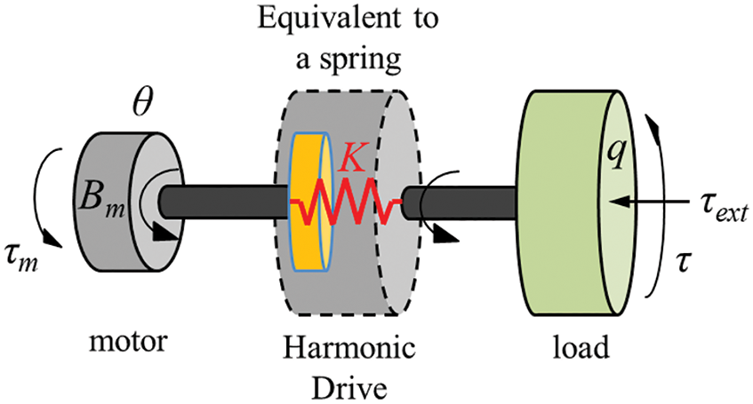
Figure 4: Equivalent torque model of the robot’s flexible joint

On the basis of the equivalence principle of flexible joints and Newton’s third law of motion, a mathematical model was used to express the interrelation of the moment transfer.

{M(q)q¨=τ+τextτ=K(θ−q)Bθ¨+τ=τm−τf.(2)

In Eq. (2), M represents the moment of inertia of the load at the end of the robot joint, and θ−q represents the rotation angle error at the motor end and connecting rod end. τ represents the torque transmitted to the link. τf represents the frictional force of robot joints. The frictional force model can be obtained through an empirical formula or parameter identification method.

When the robot moves from the static state to the moving state, enough external force is needed to offset the friction to realise the dragging and teaching of the robot. The dynamic model of the flexible joint was established as follows:

{τext=Bθ¨+M(q)q¨+τfτ=K(θ−q).(3)

Eq. (3) reveals that during dragging and teaching, the external force exerted on the joint must overcome the rotational inertia of the joint motor and the static friction when the joint moves from a static state to a moving state. To simplify the robot dragging and teaching process, the influence of system inertia and friction on the system must be reduced.

Given that the robot joint uses a harmonic reducer to grant the joint structure a certain flexibility, it can be considered that the robot was a flexible joint. On the basis of Spong’s feedback control method for flexible joint robots [12] and Albu’s full-state feedback, impedance design and experiments applicable to flexible joint robots, the dynamics model of robots with flexible joints was extended into the following form:

{M(q)q¨+C(q,q˙)q˙+G(q)=τ+τextτ=K(θ−q)Bθ¨+τ=τm−τf.(4)

Assume that the degree of freedom of the robot was n, where M(q)∈Rnxn represents the inertia matrix of the robot.

C(q,q˙)∈ Rnxn represents the robot’s Coriolis force and centrifugal force matrix.

G(q) ∈ Rn represents the gravity matrix of each joint.

q∈ Rn represents the Angle matrix of the joint output.

τ∈ Rn represents the output torque of the harmonic reducer by the flexible component of the joint.

The dynamic model of the flexible robot in Eq. (4) demonstrates that the zero-moment control of the robot was mainly affected by gravity and friction. The controller must be able to distinguish between external forces and the gravity the friction of the robot itself so that the joint actuator only responds to external forces.

3.2 Zero-Gravity Controller Design

The control law of the system controller reflects the relationship between the input/output signals. If analysed purely in the mathematical sense, a strict process of the control law can be deduced as follows: Firstly, the dynamic equation of the system was constructed, and a controller that conforms to the system model was designed. The stability function was derived by combining the two. If the Lyapunov stability is satisfied, the designed controller is correct, if the Lyapunov stability is not satisfied, the controller must be re-designed. The design process of the controller is shown in Fig. 5.

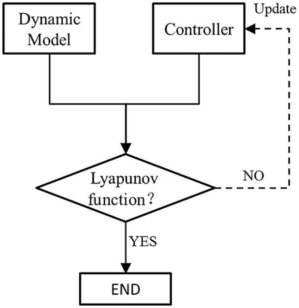
Figure 5: Design process of the controller

To achieve small external force traction in the zero-gravity control of a collaborative robot based on flexible joints, the joint controller was set in the form of the proportional controller by using the output torque τm of the motor and the output torque τ of the harmonic reducer.

τm=−Ktτ.(5)

The controller model of Eq. (5) was substituted into the mathematical model (2) of the flexible joint of the robot, and the relationship between the rotational inertia of the joint motor and the friction corresponding to the traction force was obtained

M(q)q¨+Bθ¨+τf1+Kt=τext.(6)

The comparison of Eq. (6) with Eq. (3) shows that the influence of the motor moment of inertia and friction on joint dragging was 1/(1+Kt) times of the original. In the joint control, Kt > 0 was taken, then

Bθ¨+τf1+Kt<Bθ¨+τf.(7)

Based on Eq. (7), under the same external force, the larger the value of Kt, the easier the traction will be. Extending from a single flexible joint to the whole collaborative robot system, and for the collaborative robot with n degrees of freedom, Kt can be expanded into a positive definite and triangular moment matrix, comprising n×n parameters (Kt=diag(Kt1,Kt2,⋯,Ktn)).

The controller model of Eq. (5) was substituted into the dynamics model (4) to obtain the corresponding external force value τext.

M(q)q¨+C(q,q˙)q˙+G(q)+Bθ¨+τf1+Kt=τext,(8)

At this point, if the external force τext acting on the output end of the joint was removed, that is, in Eq. (8), the angular velocity of the connecting rod was q˙=0, and the angular acceleration was q¨=0, then it can be obtained from Eq. (8).

−G(q)−(1+Kt)−1τf=Bθ¨(1+Kt)−1.(9)

According to Eq. (9), if at this time

−G(q)>(1+Kt)−1τf.(10)

Then, the robot joint will fall rapidly due to the influence of its gravity, preventing it from maintaining its current position, thus failing to achieve the zero-gravity mode. Therefore, the designed joint controller (5) fails to meet the actual control requirements.

The above analysis reveals that the influence of rotational inertia and friction on joint dragging was reduced by the controller (5) to a certain extent, but the influence of joint gravity on robot zero-moment control was not eliminated. To meet the requirement of zero-moment control, the controller must be redesigned to eliminate the influence of gravity. On the basis of the above requirements, the controller (5) was extended. The following controller was obtained.

τm=τ+Kt(G(q)−τ).(11)

Substituting the newly constructed controller (11) into Eq. (4), we can obtain

M(q)q¨+C(q,q˙)q˙+Kt−1Bθ¨+Kt−1τf=τext.(12)

Eq. (12) presents that the gravity term G(q) in the system was eliminated by the controller. At this point, if the external force τext acting on the output end of the joint was removed and the robot was maintained at the current position, the angular velocity of the connecting rod in Eq. (12) was q˙=0, and the angular acceleration was q¨=0, then it can be obtained from Eq. (12).

Kt−1Bθ¨+Kt−1τf=0.(13)

The Eq. (13) demonstrates that the larger the value of Kt, the easier the traction will be, by the controller (11). When Kt→+∞, the Eq. (13) →0, this shows that the system was progressively stable, thereby meeting the Lyapunov stability requirements, which proves that the controller design was rational. By adjusting the gain value Kt of the controller, the gain value Kt >1 thus weakens the effect of the motor rotation inertia and the friction on the dragging and teaching function, and the larger the value of the adjustment coefficient Kt, the easier the traction will be. Therefore, only the smaller external force τext can drag the robot.

3.3 Robot Parameter Identification Model Based on Least Squares

For robot system parameters identification, the theoretical basis was the same, and a mathematical model was required [13]. According to the Eq. (4), a dynamic model was established for a robot with a flexible joint. For a single link system identification, the motor output torque τm can be represented by the following kinetic equation:

τm=Bθ¨+M(q)q¨+C(q,q˙)q˙+G(q)+τf−τext.(14)

The motor output torque τm and the motor current are linear relationships, τm=Kmi, current i can be collected by the Hall sensor in the joint motor drive module. Km is the motor torque sensitivity, B is the moment of rotation of the motor, G(q) is the gravity, τf is the friction and q is the joint angle.

During parameter identification, low-speed dynamic equilibrium motion was adopted. There is no external force existed during the whole experiment (τext=0). At this time, on the basis of the Eq. (14), the kinetic equation of the single-link system was obtained

τm=Bθ¨+M(q)q¨+C(q,q˙)q˙+G(q)+τf(15)

Robot dynamics parameters-Gravity Matrix G(q) can be obtained through the parametric modelling of 3D software, so identifying the gravity matrix is unnecessary. The following transformation was made by the Eq. (15).

G(q)=Kmi−Bθ¨−M(q)q¨−C(q,q˙)q˙−τf.(16)

Many kinds of system identification methods exist, including least squares, maximum likelihood estimation, Kalman filtering method and finite element method. The most widely used and most effective in system identification is the least-squares method, and the dynamic equation will be written in the form of matrix multiplication.

G(q)=HTQ=[Km−B−M(q)−C(q,q˙)−τf]T[iθ¨q¨q˙1].(17)

According to the form of the above system dynamic equation, it can be obtained that the vector H was independent of the robot’s motion state, and parameter identification was required. The vector Q was the motion parameters of the robot joint, which was related to the motion state. Analysing the Eq. (17) unveils that when the gravity matrix G(q) and the motion parameter Q of the joint are known, obtaining vector H on the basis of the least-squares method would be effortless.

The robot adopts a dual encoder that can detect the joint location information accurately, and the robot driver with current detection modules was designed. The Hall sensor was used in the motor drive module for current detection. Typically, q˙ and q¨ can be obtained by numerical differences. However, differential operations produce great noise, which must be reduced by filtering. However, filtering will cause phase delays. The phase delay problem was eliminated by inputting the parameters on both sides of the Eq. (17) into the same filter. The vector H was a constant, and the filter processing was not affected. The key to zero-moment drag was to compensate for its gravity and friction.

Depending on the changing joint position of the robot, the current gravity G(q) of each joint was calculated, thereby controlling the motor output torque (i.e., output current) to compensate for gravity and frictional force, intensifying the fluency of the drag. Given that the robot dynamic parameters include the centroid coordinates and quality of each link, it can be calculated by a 3D software, SolidWorks, so identifying the gravity matrix is unnecessary. The gravity compensation value required for each link can be calculated directly through the Lagrangian law. Thus, the function of zero resistance dragging and teaching can be realized.

This section takes the torque sensitivity and friction of Joint 2 in Fig. 6 as an example to introduce the low-speed dynamic balance method. The heavy torque G2 of Joint 2 was obtained on the basis of the robot dynamics equation by the DH parameter. In the experiment, in addition to Joint 2, the remaining joints maintained the initial zero state of the robot. The force analysis of Joint 2 is shown in Fig. 6.

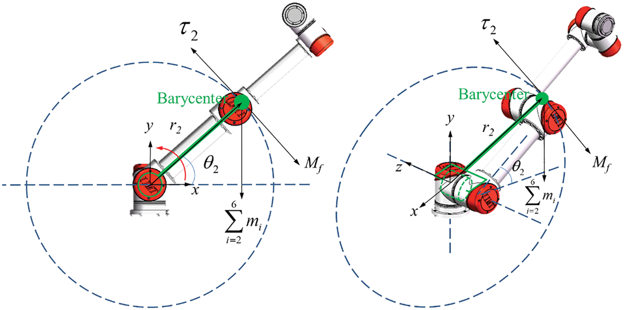
Figure 6: Force analysis of Joint 2

4  Parameter Identification Experiment

4.1 Parameter Identification Experiment Process

Low-speed dynamic balance movement was adopted for parameter identification. During the movement, the angular acceleration of the motor end was θ¨=0, the angular velocity of the connecting rod end was q˙=0 and the angular acceleration was q¨=0. No external force existed during the process (τext=0). At this time, on the basis of the Eq. (16), the dynamic equation of the single-link system, as shown below, was obtained:

G(q)=HTQ=[Km−τf]T[i1].(18)

MATLAB was used to simulate the robot motion planning. Joint 2 of the robot moved and rotated at a low speed on the basis of the planned motion, whereas other joints maintained the initial state of the robot. Given that the planned movement was low-speed rotation, and it was close to the uniform movement, it ignored the effects of the torque value brought about by the rotational inertia B of the robot joint itself. The force of friction was approximately static friction τf. At any moment during the motion, the torque balance equation of the sections of the joints and connectors above Joint 2 was

τ2=∑i=26migTri+τf.(19)

where mi was the quality of the link i. The mass of the centre was the sum of the mass of all joints above Joint 2 (including Joints 3–6) and the connecting rod. r2 was the position vector of the centre of mass p in the Joint 2 coordinate system.

Assume that the generalized coordinate of Joint i was θi. In this experiment, r2 was only related to θ2 (the remaining joint rotation angle θ1,θ3,θ4,θ5,θ6 all are 0). θ2 indicates that the rotation angle of the robot Joint 2 can be read directly by the joint encoder. τ2 was the output torque of Joint 2 after deceleration, and the torque was improved by the harmonic reducer, which can be expressed as τ2=100Km2i2. The deceleration ratio of the harmonic reducer used in the joint was 100, and the torque sensitivity of the motor was assumed to be Km2. The current during the rotation of Joint 2 was recorded as i2. τf was the friction torque of the joint in the process of rotating at a low speed, which was approximately the maximum static friction torque.

This experiment adopts the parameter identification method of torque sensitivity and friction under low-speed dynamic balance. Let the motor of Joint 2 rotate at a low speed in position mode. The joint positions and motor current values during the whole movement were collected as excitation signals of the system and input into the parameter identification equation.

When the robot joint rotates at a low speed, it can approximately satisfy the torque balance equation. During the whole movement, robot Joint 2 always rotates at a low speed. It can be assumed that the friction torque τf was approximately constant, and the Eq. (19) can be written as follows:

100Km2i2=Mgf(θ2)+τf(20)

The Eq. (20) was rearranged to obtain the following equation:

Mgf(θ2)=100Km2i2−τf(21)

In the Eq. (21), Mg was the gravity moment of Joint 2, the friction torque τf was approximately constant, and there existed a linear relationship between the current i2 and θ2. By collecting the data of the current value i and the rotation angle of the joint θ2, the linear equation can be identified by the least square method.

As a result, the values of torque sensitivity km2 and friction torque τf were obtained. The steps of the identification experiment are as follows.

According to the motion range of Joint 2, the joint trajectory was planned with the expected reciprocating low-speed motion, and the spline programming method was used for interpolation. Acceleration and deceleration in the starting and commutation area of the joint motion are conducted, which will move at a low speed in the rest of the state, as shown in Fig. 7.

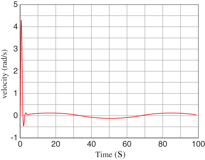
Figure 7: Joint velocity curve

The robot joint was set to reciprocate at a low speed, and the maximum speed in the whole process was roughly 2 degrees per second (joint axis). The current value i and rotation angle θ2 of robot Joint 2 were collected in the 100 s control period, which is the excitation signal of the parameter identification. The sampling period was 10 ms, and the variation curve of joint acceleration with time is shown in Fig. 8.

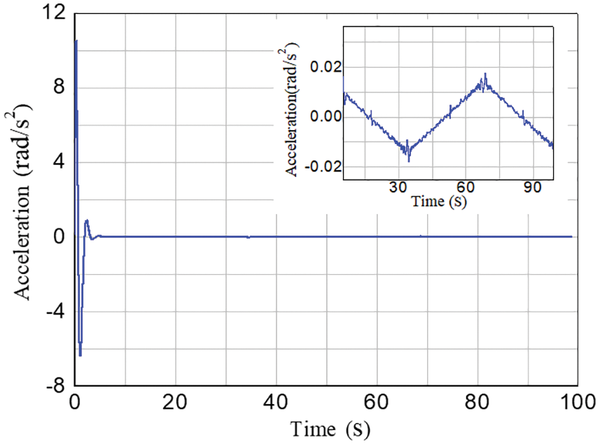
Figure 8: Joint acceleration curve

4.2 Identification Results and Verification of Torque Sensitivity Coefficient and Static Friction

The parameter identification experiment was carried out on the basis of the above two steps. The data of the current value i and the rotation angle θ2 of Joint 2 during the motion were collected. The collected data were analysed and processed. Firstly, the curve of the rotation angle θ2 of Joint 2 and the change of current value i with time were drawn, as shown in Figs. 9 and 10.

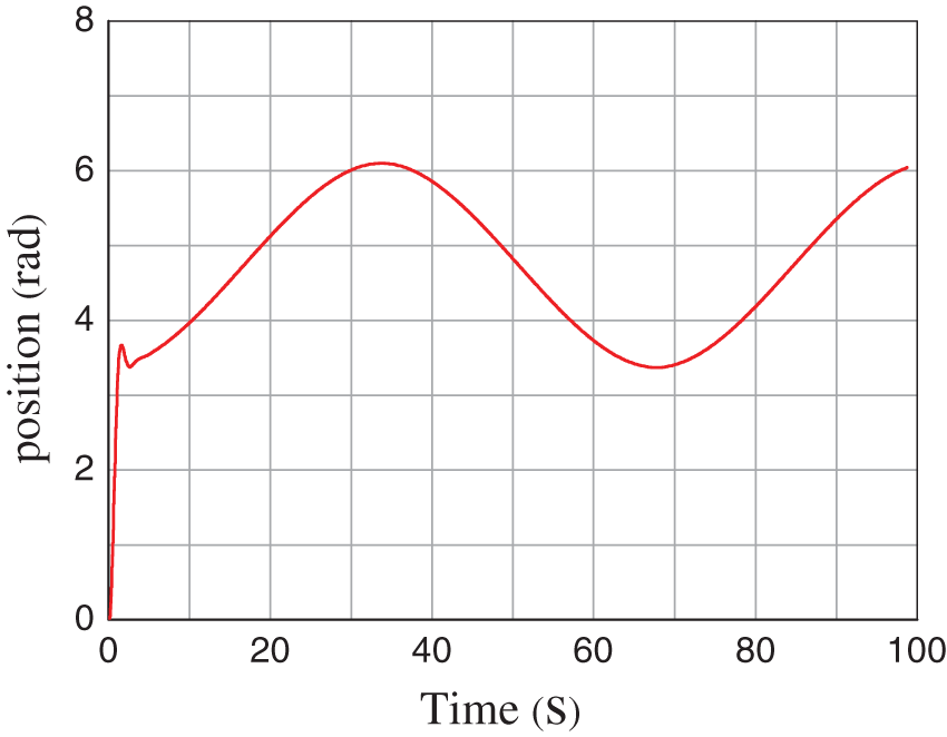
Figure 9: Curve of joint angle θ2

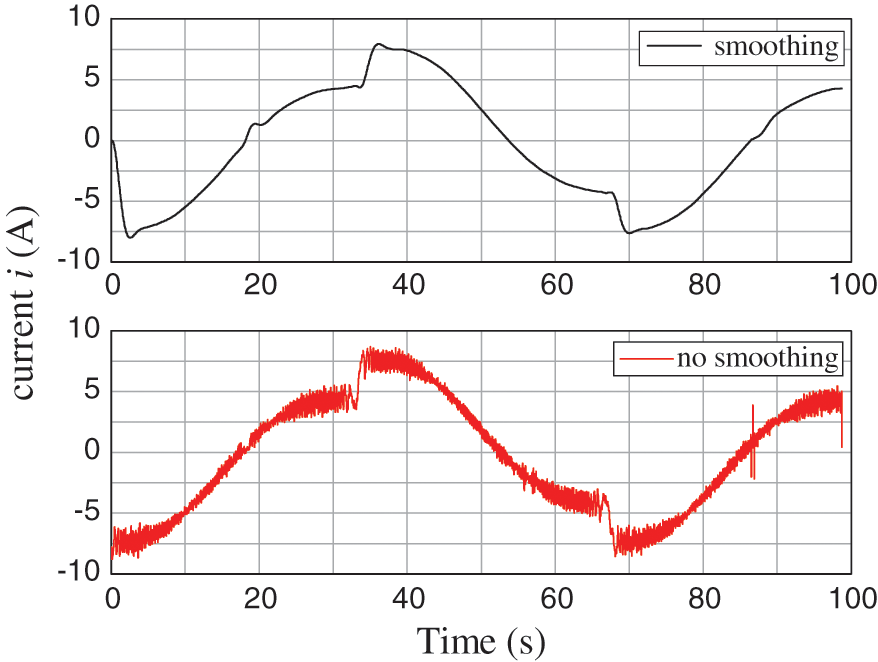
Figure 10: Curve of joint current

On the basis of the experiment, the motor current and angle changed when the positive and negative rotation of Joint 2 were taken, and the relationship between them is shown in Fig. 11.

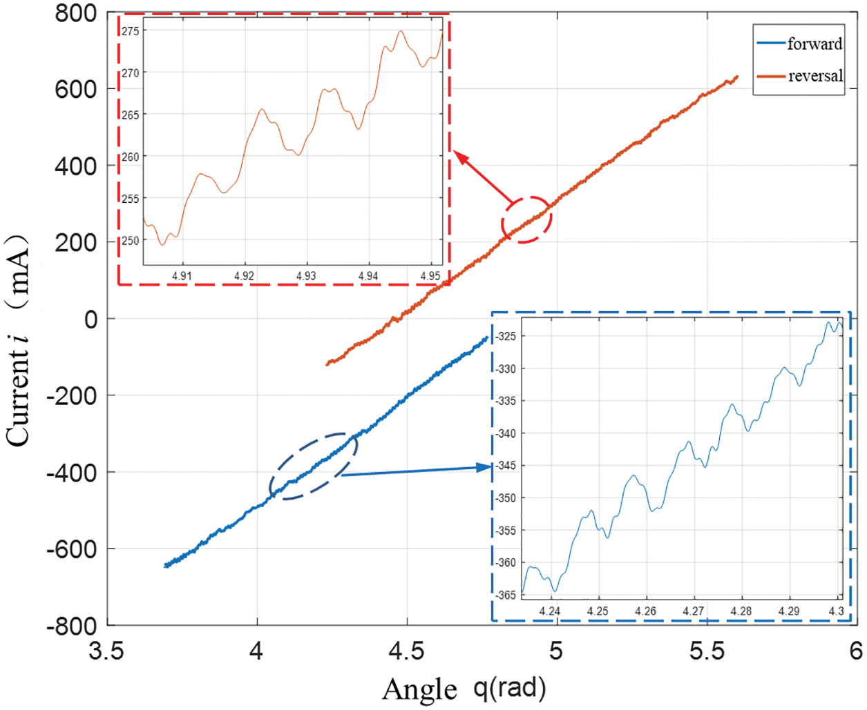
Figure 11: Relationship between the current and angle change values

Fig. 9 shows that the joint velocity changes with time. The speed of the robot joint changed minimally and was basically in a state of uniform motion. On the basis of the speed change, the gravity torque and motor current under uniform motion were selected, and the straight line was fitted on the basis of the relationship between the collected gravity moment and motor current value, as shown in Figs. 12 and 13.

Figure 12: Fitting curves of heavy moment G and current i under forwarding rotation

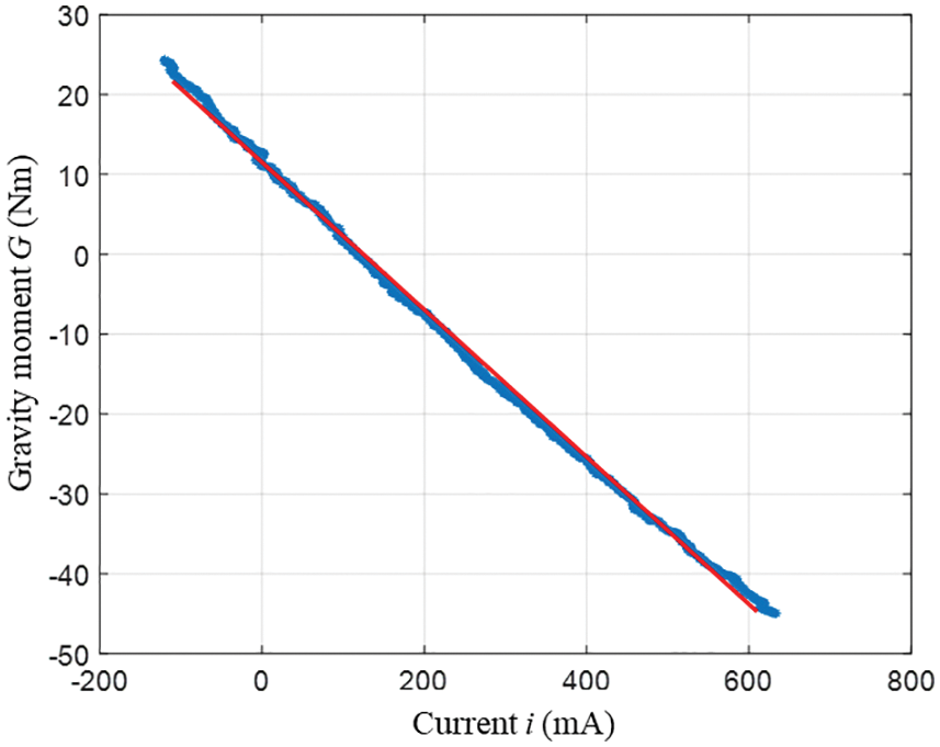
Figure 13: Fitting curves of heavy moment g and current i under rotation

Finally, the estimated values of torque sensitivity and friction torque of Joint 2 in the case of positive rotation are 0.0874 Nm/An and 8.1200 Nm, respectively. The corresponding straight-line equation is

Mgf(θ2)=8.74i−8.1200.(22)

In the case of reversal, the estimated values of torque sensitivity and friction torque of the motor are 0.0922 Nm/An and −11.5242 Nm, respectively. The corresponding linear equation is

Mgf(θ2)=9.22i+11.5242.(23)

From the estimated value of motor torque sensitivity and friction torque identified in the case of the positive and negative rotation of Joint 2, the estimated value of motor torque sensitivity was roughly 0.09 Nm/An, but a certain difference existed in the friction in the process of positive and negative rotation of Joint 2, so the smooth dragging and teaching function can be realised, and the compensation of Joint 2 can be set as follows:

Mgf(θ2)=9i+τf.(24)

Given the difference of friction during the positive and negative rotation, the following expression of friction torque can be obtained

τf={8.1200,ifθ˙2>vlim−11.5242,ifθ˙2<−vlim0,if−vlim<θ˙2<vlim.(25)

vlim was a preset critical value of speed after the robot entered the teaching mode. On the basis of the experiment, the upper limit of the speed was set to approximately 3 deg/s, because extremely low speed will lead to the vibration of the manipulator.

When the robot was in a teaching mode, once the speed of the robot’s joint exceeds this preset value, it means that the operator begins to drag the robot. At this time, the compensation value of friction must be added.

The traditional small and medium-sized collaborative robot can realise zero-moment drag teaching on the basis of the torque compensation control without using an external force sensor. The key technology was the compensation of gravity torque and friction of the robot joint. On the basis of the parameter identification method of robot torque sensitivity and friction based on low-speed dynamic balance, the parameter estimation of motor torque sensitivity can be realised in a certain precision range, and the joint friction torque can be identified simultaneously. The free drag of the robot can be easily realised by compensating gravity torque and friction torque in real time.

In this chapter, on the basis of the dynamic model, the key compensation value of the robot joint was solved by the robot single joint parameter identification method, and finally, the robot drag teaching was realised.

5  Experiment of Dragging and Teaching Function and Trajectory Repetition

This part is mainly for experimental verification for the torque compensation control. The experimental purpose was to verify the reliability of collaborative robot joint structure, the feasibility of zero control algorithm. Dragging and teaching experiments in torque compensation mode verified the accuracy of dynamic modelling and friction parameter identification.

The zero-moment control technology of robot torque compensation is mainly used in robot dragging and teaching. To realise the easy dragging, the torque value of the robot’s joint compensation must be calculated in real-time. The key to zero-moment drag was to compensate for the two dynamic parameters of gravity and friction.

The current gravity term G(q) of each joint was calculated based on the changing positions of the robot. By controlling the output torque (output current) of the motor to realise the compensation of gravity and friction to make the drag smoother. According to the structural characteristics of the robot, the mass of each connecting rod of the robot is m1, m2, m3, m4, m5 and m6, respectively, as shown in Fig. 14. The mass matrix of each connecting rod mi (i = 1 ~ 6) was

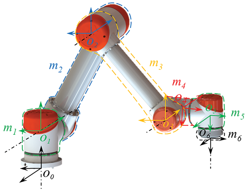
Figure 14: The mass distribution of the robot

m=[m1m2m3m4m5m6]=[3.758.242.41.461.460.2].

The compensating torque of joint gravity can be calculated by using the dynamic equation. The gravity torque compensation function of each connecting rod of the robot was

G1=0

G2=−40.87cos⁡(q2)−18.64cos⁡(q23)−0.35cos⁡(q234)sin⁡(q5)+1.69cos⁡(q23)sin⁡(q4)+1.69sin⁡(q23)cos⁡(q4)

G3=−18.64cos⁡(q23)−0.35cos⁡(q234)sin⁡(q5)+1.69cos⁡(q23)sin⁡(q4)+1.69sin⁡(q23)cos⁡(q4)

G4=−0.35cos⁡(q234)sin⁡(q5)+1.69cos⁡(q23)sin⁡(q4)+1.69sin⁡(q23)cos⁡(q4)

G5=−0.35cos⁡(q234)sin⁡(q5)

G6=0

The current compensation of the gravity torque can be calculated by Ig=Gx/Km [13].

The joint friction torque can be obtained through dynamic modelling and parameter identification. The static friction of each joint of the robot was obtained by the method in Section 4.2, which was transformed into the compensation current produced by the system to overcome the static friction through the equation If=τf/Km.

It is difficult to completely establish the robot joint friction model, and approximate modeling is generally adopted. Friction mainly includes static friction, viscous friction, and Coulomb friction. The static friction torque is the main research object in this paper because static friction torque is the most important part of the robot friction torque compensation. Compensating for viscous friction and Coulomb friction is mainly to make the robot smoother when dragging. Static friction torque has a linear relationship with the current generated by static friction torque, and the proportional coefficient is the torque constant Km of the motor. This work has been described in detail in the author’s previous paper [14]. The current to compensate for the friction can be got from the equation If=τf/Km.

The stability analysis is more important in the entire closed-loop control system. When the robot is dragged and taught at a low speed, the compensation current calculated according to the torque compensation control algorithm can perfectly overcome gravity and friction. However, in the actual teaching process, it is inevitable that the dragging speed is too fast. At this time, due to the influence of the motor’s back electromotive force, the compensation current calculated according to the torque compensation control algorithm cannot meet the robot’s dragging and teaching process. At this time, the compensation current value meets the following process:

I=Is−KbwRm.(26)

where, Kb is the motor’s counter electromotive force, w is the motor’s angular velocity, and Rm is the motor resistance. The compensation current value obtained according to Eq. (26) can satisfy the dragging process at any speed.

To verify the accuracy of the algorithm, the 6DOF collaborative robot was used as the experimental platform for zero-moment dragging and teaching. The robot can easily realise the dragging and teaching function in the zero-torque mode. To show the superiority and practicability in the zero-torque mode, three positions p1, p2, and p3 were dragged randomly during the experiment, as shown in Fig. 15.

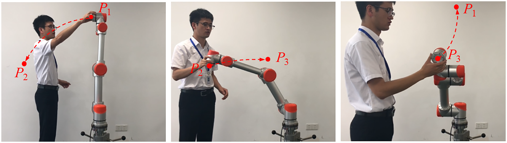
Figure 15: Robot drags to teach

The absolute position encoder of the robot was used to record the three-position points in the process of dragging. After completion of dragging and teaching, the planned linear interpolation or circular interpolation mode in the system was called to connect the trajectories of the three points smoothly. Fig. 16 shows the trajectory of the smooth transition with circular interpolation mode.

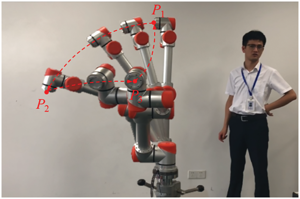
Figure 16: Robot trajectory reconstruction

As can be seen from Fig. 16, the robot can perfectly reproduce the trajectory, and the cyclic motion of the robot can be realised after setting the reciprocating motion. The analysis of the experimental results reveals that the zero-moment control algorithm based on torque control realised the zero-moment dragging and teaching of the robot by obtaining the compensation of gravity torque and friction.

6  Conclusion

The experimental results show that, compared with the traditional zero-moment control algorithm based on position control, the zero-moment control algorithm based on torque compensation control abandons the torque sensor. The accurate compensation torque was obtained through dynamic modelling and parameter identification. When the robot was dragged, the system can calculate the compensation current in real time and send it to each joint motor to overcome the gravity torque and friction. The robot can easily be dragged by overcoming its inertia force, which simplifies the whole robot system, making the teaching process simple and flexible. Ultimately, this study provides new ideas and methods for torque compensation control of all kinds of light collaborative robots.

Funding Statement: This work supported by the National Natural Science Foundation of China (52005316, 61903269, 52005317) and the Major Research and Development Program of Jiangsu Province (BE2020082-3).

Conflicts of Interest: The authors declare that there have no conflicts of interest to report regarding the present study.

References

1. Yang, C. G., Jiang, Y. M., He, W., Na, J., Li, Z. J. et al. (2018). Adaptive parameter estimation and control design for robot manipulators with finite-time convergence. IEEE Transactions on Industrial Electronics, 65(10), 8112–8123. DOI 10.1109/TIE.2018.2803773. [Google Scholar] [CrossRef]
2. Jin, H. Z., Liu, Z. X., Zhang, H., Liu, Y. B., Zhao, J. (2018). A dynamic parameter identification method for flexible joints based on adaptive control. IEEE/ASME Transactions on Mechatronics, 23(6), 2896–2908. DOI 10.1109/TMECH.2018.2873232. [Google Scholar] [CrossRef]
3. Urrea, C., Pascal, J. (2018). Design, simulation, comparison and evaluation of parameter identification methods for an industrial robot. Computers & Electrical Engineering, 67, 791–806. DOI 10.1016/j.compeleceng.2016.09.004. [Google Scholar] [CrossRef]
4. Ni, H., Zhang, C., Hu, T., Wang, T., Chen, Q. et al. (2019). A dynamic parameter identification method of industrial robots considering joint elasticity. International Journal of Advanced Robotic Systems, 16(1), 1–11. DOI 10.1177/1729881418825217. [Google Scholar] [CrossRef]
5. Jia, J., Zhang, M., Zang, X., Zhang, H., Zhao, J. (2019). Dynamic parameter identification for a manipulator with joint torque sensors based on an improved experimental design. Sensors, 19(10), 2248. DOI 10.3390/s19102248. [Google Scholar] [CrossRef]
6. Li, Y., Wang, D., Zhou, S., Wang, X. (2021). Intelligent parameter identification for robot servo controller based on improved integration method. Sensors, 21(12), 4177. DOI 10.3390/s21124177. [Google Scholar] [CrossRef]
7. Xiao, J., Zhang, Q., Hong, Y., Wang, G., Zeng, F. (2018). Collision detection algorithm for collaborative robots considering joint friction. International Journal of Advanced Robotic Systems, 15(4), 1–13. DOI 10.1177/1729881418788992. [Google Scholar] [CrossRef]
8. Michalos, G., Spiliotopoulos, J., Makris, S., Chryssolouris, G. (2018). A method for planning human robot shared tasks. CIRP Journal of Manufacturing Science and Technology, 22, 76–90. DOI 10.1016/j.cirpj.2018.05.003. [Google Scholar] [CrossRef]
9. Zhang, S., Wang, S., Jing, F., Tan, M. (2019). A sensorless hand guiding scheme based on model identification and control for industrial robot. IEEE Transactions on Industrial Informatics, 15(9), 1–10. DOI 10.1109/TII.2019.2900119. [Google Scholar] [CrossRef]
10. Gaz, C. R., Cognetti, M., Oliva, A. A., Robuffo Giordano, P., de Luca, A. (2019). Dynamic identification of the Franka Emika Panda robot with retrieval of feasible parameters using penalty-based optimization. IEEE Robotics and Automation Letters, 4(4), 4147–4154. DOI 10.1109/LRA.2019.2931248. [Google Scholar] [CrossRef]
11. You, Y. P., Zhang, Y., Li., C. G. (2014). Force-free control for the direct teaching of robots. Journal of Mechanical Engineering, 50(3), 10–17. DOI 10.3901/JME.2014.03.010. [Google Scholar] [CrossRef]
12. Spong, M., Khorasani, K., Kokotovic, P. (1987). An integral manifold approach to the feedback control of flexible joint robots. IEEE Journal on Robotics and Automation, 3(4), 291–300. DOI 10.1109/JRA.1987.1087102. [Google Scholar] [CrossRef]
13. Stürz, Y. R., Affolter, L. M., Smith, R. S. (2017). Parameter identification of the KUKA LBR iiwa Robot including constraints on physical feasibility. IFAC-PapersOnLine, 50(1), 6863–6868. DOI 10.1016/j.ifacol.2017.08.1208. [Google Scholar] [CrossRef]
14. Chen, S., Luo, M., Jiang, G., Abdelaziz, O. (2018). Collaborative robot zero moment control for direct teaching based on self-measured gravity and friction. International Journal of Advanced Robotic Systems, 15(6), 1–11. DOI 10.1177/1729881418808711. [Google Scholar] [CrossRef]
Cite This Article
Copyright © 2023 The Author(s). Published by Tech Science Press.
This work is licensed under a Creative Commons Attribution 4.0 International License , which permits unrestricted use, distribution, and reproduction in any medium, provided the original work is properly cited.
Downloads
Citation Tools