Classification of Human Protein in Multiple Cells Microscopy Images Using CNN

1  Introduction

Proteins are located in a specific location to perform a particular function within the cell. Proteins perform various physiological processes supporting human life [1,2]. The Knowledge of protein locations in the cell is necessary to understand the protein-specific function and the overall organization of the cell. Different subcellular distributions of proteins can lead to heterogeneity of function between cells. An overview of human cells is shown in Fig. 1. The analysis of these differences is essential to perceive the cells’ function, discover diseases, develop treatments, and enhance the drug industry. Human proteins have high importance in human cells.

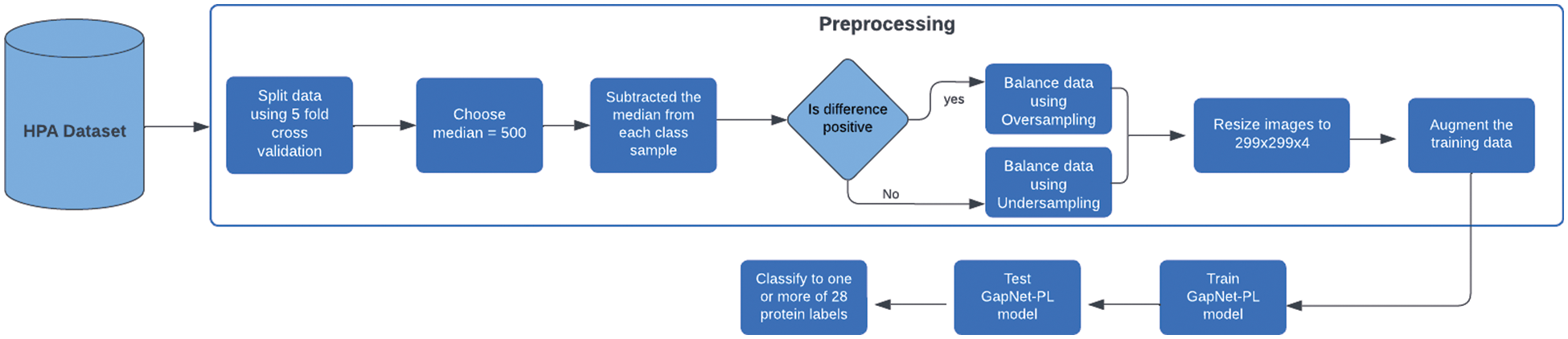
Figure 1: Overall flow of the proposed architecture

In contrast, the subcellular localization of each protein can give researchers valuable information about the objective and the construction of the protein within a cell. This topic has become important in the current research of biological processes because of its essential role in pathology studies in the pharmaceutical industry. A deep understanding of the cell organelles in which the protein exists can participate in multiple biological processes, help to detect various diseases and develop appropriate treatments [3–5].

Protein localization is the process by which a protein gathers in a specific site. The prediction of protein focuses on determining the unknown sites of the protein. There are two methods for predicting subcellular protein localization (PSL): 1D sequence-based and 2D image-based methods. The image-based 2D method is used to overcome the limitations of the 1D sequence-based approach [6]. Classifying the mixed pattern of proteins and different types of human cells is required [7].

To identify all human proteins found in cells, tissues, and organs, a program called the Human Protein Atlas started in 2003. The HPA program provided large datasets of high-throughput microscopy images of human proteins [8]. Many Kaggle competitions have been held using these datasets.

In several areas of medical and bioinformatics, the analysis of the computerized microscopy image plays a significant role in computer-aided prognosis. Manual analysis and evaluation of these images are difficult. Recently, deep learning algorithms have proven to be an effective tool for processing and analyzing microscopy images, including nuclei recognition, cell segmentation, tissue segmentation, image classification, and other tasks. Convolutional neural networks (CNNs) are a common type of deep learning architecture [7].

Despite recent developments in the analysis of microscopy images using CNN architectures, classification models have faced considerable difficulties reaching high performance because most protein subcellular images have a huge class imbalance. Also, there is a lack of studies that use and compare multiple types of activation functions in deep learning algorithms. The contribution of the paper is to improve the performance of the research which uses the same data, combining oversampling and undersampling methods to solve the data imbalance rather than using only oversampling, and trying a powerful activation function PReLU which has not been used before in protein classification tasks.

This paper used oversampling and undersampling methods to address the data imbalance issue. We applied a CNN model known as GapNet-PL [9] to solve the multi-label classification task based on a Human Protein Atlas Classification (HPA) dataset [10]. This study shows that the PReLU activation function-based model can outperform the SeLU activation function-based deep learning model and get higher results for the most used metrics.

We demonstrated that the oversampling and undersampling methods could balance the dataset classes and improve classification accuracy. The PReLU activation function-based model achieved an average of AUC equal to 0.896, an F1 score of 0.541, and a recall of 0.473 on the test dataset. While SeLU was better in the rest of the metrics and gave an accuracy average of 0.495 and a precision average of 0.705.

The remainder of this paper is structured as follows: A background and related work are provided in Section 2. Section 3 describes the dataset, the classification model, and the evaluation metrics used. Section 4 discusses the experimental setup and configurations of the deep learning model. The results and discussion are given in Section 5. Finally, this research is concluded in Section 6 with a brief explanation for future work.

2  Background and Related Work

Human cells can generate massive medical and microscopy images sufficient to train deep-learning models. Therefore, deep learning techniques will replace the traditional method of evaluating and analyzing complicated biological images [11]. Convolutional neural networks (CNN) have effectively analyzed different types of biological and medical images. A study by Esteva et al. [12] demonstrated how skin lesions could be classified using a CNN, which was trained from images utilizing only pixels and disease labels as inputs. For the first time, CNN’s diagnostic abilities were evaluated by Haenssle et al. [13] with those of a broad worldwide group of dermatologists and professionals. CNN consistently outperformed dermatologists’ diagnoses. The artificial jellyfish’s intelligent living behavior is used to improve ANN. This classifier, also known as JellyfishSearch_ANN, is used for precisely classifying cervical cancer [14]. Microscopic blood slides have been used to measure parasitemia using image analysis by CNN to improve diagnosis [15].

Deep learning models have recently been proven to be very successful in classifying microscopy images and predicting human proteins rather than traditional machine learning techniques. The convolutional neural network (CNN), a deep learning architecture, is widely used to replace machine learning algorithms in classifying high-throughput microscopy data [16,17]. Although traditional machine learning methods use only hand-crafted features extracted indirectly from protein primary sequences, deep learning classifiers can automatically discover and extract useful feature representations, such as non-linear feature correlations, which allows enhancing the prediction accuracy. The results showed that DeepPSL works better in prediction [18]. Another model called DeepYeast, presented by Hu et al. [19] outperformed the support vector machine (SVM) in classifying eight subcellular localizations of protein images. The accuracy of the DeepYeast was 47.31% compared to the SVM (accuracy of 39.78%). The deep convolutional neural network (DeepLoc) model was proposed to analyze images of yeast cells to classify protein subcellular localization and achieved an accuracy of 72% [20].

While high-quality images consume memory and need a long processing time, Rumetshofer et al. [9] presented a low-cost and time-efficient CNN architecture called GapNet-PL. This model has three layers and uses a global average pooling layer where hints can be collected at low-level convolutions. While high-resolution images need a large memory, they used the SeLU activation function to reduce memory consumption. This model has been compared to many other models, such as DenseNet, DeepLoc, FCN-Seg, etc. GapNet-PL performed better than other models, giving an AUC of 98% and an F1 score of 78%. Customized architectures for the multi-label classification of human protein proposed in Zhang et al. [21] study outperformed the previous architecture (GapNet-PL) [9] by more than 2% in the F1 score.

Mitra [22] emphasized that oversampling is essential to enhance model performance and learning for classifying protein in multi-label microscopy images with a huge data imbalance. Protein classification task was integrated as a minigame in a mainstream video game (EVE Online) called Project Discovery [23]. They developed an automatic cellular annotation tool to localize proteins divided into 29 subcellular localization patterns. They used transfer learning to achieve an F1 score of 0.72 by integrating deep learning and gamer annotations. Two types of CNNs are used for the protein classification task, a CNN architecture and a fully convolutional network. When comparing the two networks, FCN outperforms CNN [24]. Two main approaches are used by [5] to classify the human protein atlas images. The first approach uses the conventional image feature extraction method and the Random Forest algorithm as a classifier. The second approach uses two CNN models, Hybrid Xception and ResNet50. The result of the Hybrid Xception is 0.69 for the F1 score, 0.41 for ResNet50, and 0.61 for the conventional approach. ResNet pre-trained model achieved an F1 score of 0.3459 for the protein classification task using the HPA dataset [25]. Tu et al. [26] proposed a new method called SIFLoc, containing two main stages. The first is self-supervised pre-training which uses a hybrid data augmentation method and a modified contrastive loss function. The second stage applies the supervised training.

Data imbalance is one of the most significant barriers to the high performance of protein classification models. Rana et al. [27] have suggested using oversampling to handle the multilabel data imbalance in the protein localization task.

A composite loss function built by [2] merged focal loss and Lovasz-Softmax loss in training. They used CNN pre-trained models in protein classifications; the models were SE-ResNeXt-50, DenseNet-121, and ResNet50. They achieved an F1 score equal to 0.5292 in the testing dataset. Another essential component of artificial neural network training is selecting an activation function. The choice of the activation function plays a vital role in the neural network performance. In a study by Jiang et al. [28], PReLU was combined with a CNN architecture called AlexNet, for target recognition. Using PReLU improves performance and makes the model achieve an accuracy of 84.02%. Wang [2] and Adweb et al. [29] used the PreLU activation function for medical image classification. Furthermore, researchers have developed multiple novels and effective optimization strategies to handle the optimization problem of the training [30].

The limitations of the previous works can be summarized as many papers have been published on predicting multi-label protein using customized architectures [9,18,21]. Some researchers have focused on outperforming hand-crafted machine learning algorithms such as SVM [18] rather than improving the existing deep learning models. Despite the effectiveness of the PreLU activation function in classifying images, there is a lack of research that uses PreLU in the protein classification task. While the biggest concern of protein classification models is data imbalance, most papers use oversampling [19,22,27]. That can lead to an increase in data size and ultimately challenges the model training.

The main objective of this research is to solve the imbalance problem of the HPA dataset by combining both oversampling and undersampling techniques to enhance the accuracy of the classification of protein microscopy images. Furthermore, we have examined the ability of the PReLU activation function to produce precise annotations of the subcellular localization for thousands of human proteins in multiple-cell images.

3  Methodology

In this paper, we will use a CNN model called GapNet-PL. Preprocessing consists of two steps: resize the images to 299 × 299 × 4 and then apply the oversampling and under-sampling techniques to remove the data imbalance. The whole dataset is divided using the K-fold cross-validation method into 5 folds. We have five models in total, and one fold is used as a validation fold while the rest is used for training. After finishing the training of all models, we will average their results to get the final result of the GapNet-PL model. The proposed architecture of the methodology is shown in Fig. 1.

3.1 Human Protein Atlas Image Classification Dataset

This data was presented by the HPA team and released for the Kaggle competition called Human Protein Atlas Image Classification [10]. Fig. 2 shows a sample of images of different classes. It has 27 distinct cell types with vastly diverse morphologies, all impacting the protein patterns of the various organelles. This dataset has 31072 images in the train.csv file having a size of 512 × 512 pixels. The dataset images are represented by four filters (RGBY): red for microtubules, green for the protein of interest, blue for the nucleus, and yellow for the endoplasmic reticulum. For example, a display of different channels in the image with an ID equal to 1 is shown in Fig. 3.

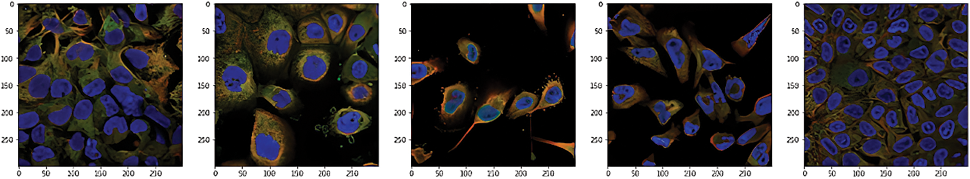
Figure 2: Sample of the dataset

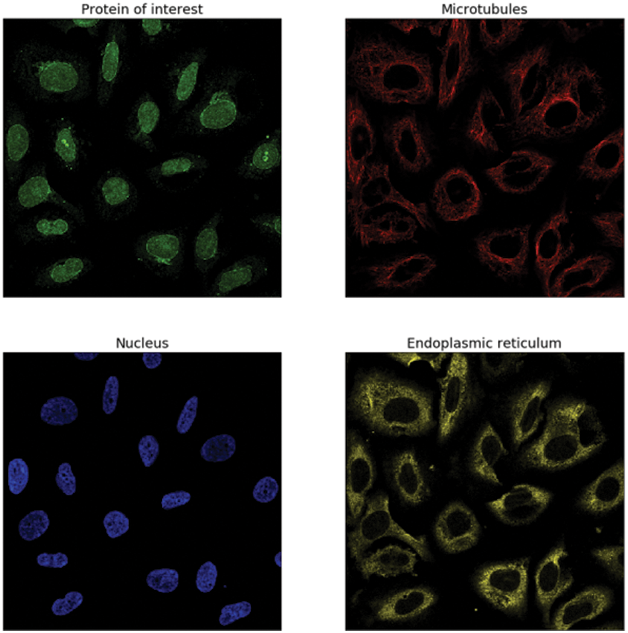
Figure 3: The image with ID == 1 has the following labels: 7, 1, 2, 0, and these labels correspond to (Golgi apparatus, Nuclear membrane, Nucleoli, and Nucleoplasm)

3.2 Data Preprocessing

For data preprocessing, we resized the images to 299 × 299 × 4. These numbers refer to the length, width, and image channel. We chose a smaller image size than the original because training the smaller images will be faster and converge more quickly.

Many methods exist in the literature to solve the problem of data imbalance. Two techniques are used in this paper to handle the data imbalance: the oversampling method and the under sampling method. Oversampling reduces the negative effect of the skewed distribution of data by duplicating samples from the minority classes, so that the number of examples in each class is equal to or nearly identical. In contrast, the under sampling technique reduces the negative effect of the skewed distribution of data by randomly removing samples from the majority classes. Combining the over-sampling and under-sampling techniques are called the hybrid method [31–33].

In this paper, we use both over-sampling and under-sampling to handle the imbalance problem. The true median equals 715 between class samples, but we chose 500 as a median value because it gave a better class distribution. Then, we tried to approximate the samples to be equal or closer to that value. To do that, we subtracted the median from each class sample and made a condition. If the difference is positive, we will use oversampling and duplicate samples of that class using the resulting number. Otherwise, if the difference is negative, we will do the opposite, which is the under-sampling, and remove the resulting number from that class sample. After applying that, there is still an unbalance problem because each class will affect the other classes. However, the distribution has improved significantly. We used the augmentation method for the training set to avoid overfitting and increase the model’s generalizability. Data augmentation techniques are geometric transformations, color space transformations, and Kernel filters. In this paper, geometric transformations are used on the oversampled data. One of the following geometric transformations is randomly applied on each image, rotation by (0, 90, 180, 270) and flipping horizontally or vertically [34].

3.3 CNN Model Architecture

GapNet-PL is a CNN model with a two primary steps approach. The first step is an encoder designed to handle high-throughput microscopy images. The encoder has multiple convolutional layers; some have a stride of 2 max-pooling layers implemented to learn abstract features at various spatial resolutions. The second step uses global average pooling to reduce the feature maps from three layers to one-pixel size and concatenate the resulting feature vectors. This pooling layer can also help to reduce the impact of weak labels. The resulting feature passed into a fully connected network of two hidden layers for the final classification. GapNet-PL uses the SeLU activation function with normalization rather than the Rectified Linear Unit (ReLU) for practical training to minimize memory usage [9]. We illustrated the GapNet-PL architecture in Fig. 4.

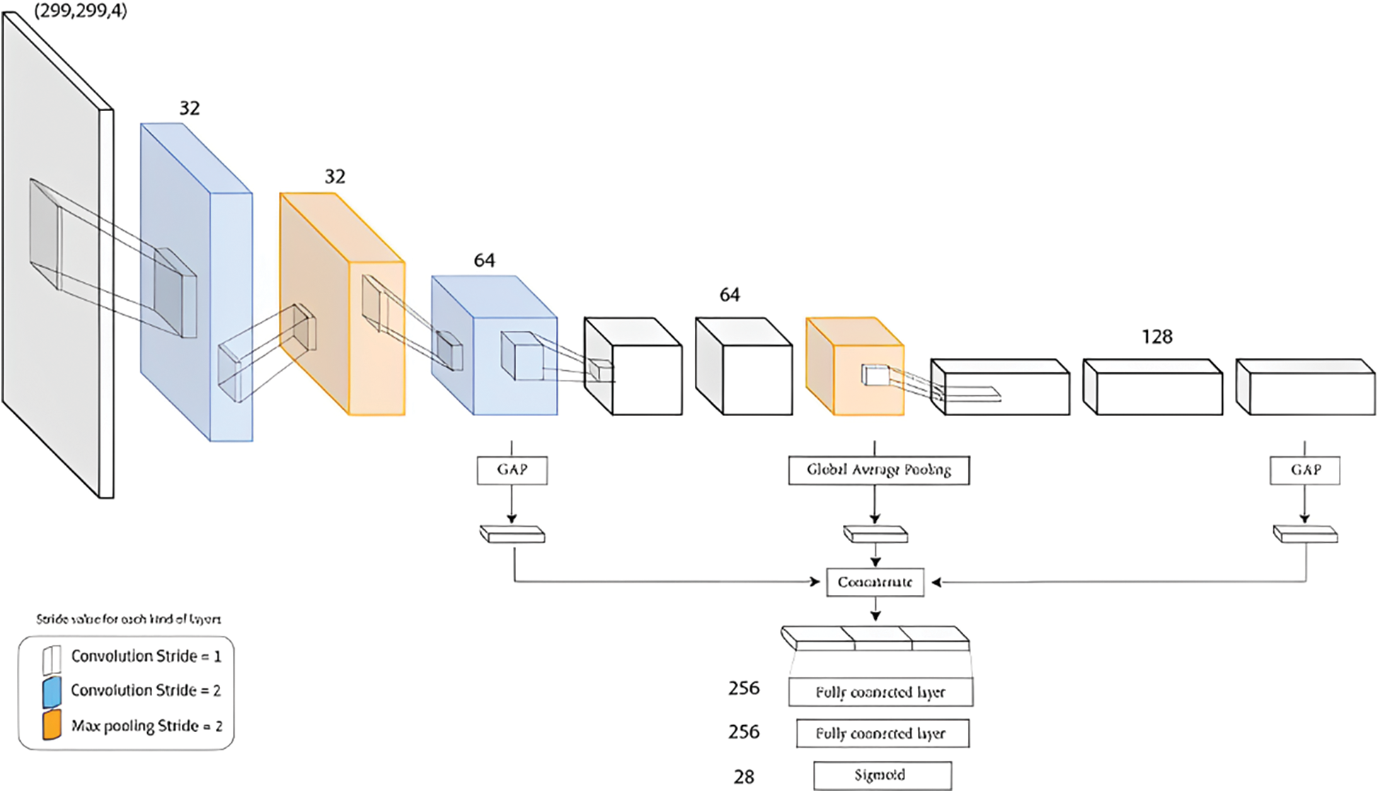
Figure 4: GapNet-PL Architecture

This paper highlights the significance of the activation function and its impact on the neural network’s performance. Moreover, we compare the same architecture using two different activation functions: the SeLU activation function and Parametric Rectified Linear Unit (PReLU). PReLU is a generalized version of the standard Rectified Linear Unit (ReLU). With almost no additional computational effort and no overfitting risk, PReLU is an activation function with a slope for negative values which generalizes the typical rectified unit; it enhances model fitting [35].

f(yi)={yi,if yi>0aiyi,if yi≥0(1)

The SeLU activation function provides self-normalization at the neuron level and can adapt to sudden changes. The SeLU activation function is good for the neural networks of the denser layers, but it is not a good choice for convolutional neural networks. PReLU activation function can be used in convolutional deep neural networks and can avoid over-fitting. But there is no definite reason for choosing between SeLU and PReLU activation functions that always work. Hence, comparing the performance of both activation functions in a problem domain will decide which one is performing better for a particular problem domain.

3.4 Evaluation Metrics

Classification of protein in cells has been evaluated using four following performance matrices: AUC, accuracy, F1 score, precision, and recall. True Positives (TP) are the number of cases when positive labels are predicted as positive. In contrast, False Negative (FN) is the number of instances where positive labels are predicted as negative class. Similarly, True Negative (TN) and False Positive (FP) are defined for negative instances. Accuracy is defined as the ratio of correct predictions and total predictions as follows:

Accuracy=TP+TNTP+FP+FN+TN(2)

Precision is calculated as the ratio of true positive and all instances predicted as positive.

Precision=TPTP+FP(3)

The recall, also called sensitivity, is the ratio of the true positive and all positive instances in the dataset. It determines the sensitivity of the model and is calculated as follows,

Recall=TPTP+FN(4)

We defined the F1 score as a single score including recall and precision:

F1score=2(precision)(recall)precision+recall(5)

Another classification performance measurement is the AUC (Area Under The Receiver Operating Characteristics Curve) used at different threshold settings. The AUC indicates the degree or amount of separability, whereas the ROC is a probability curve that shows how well the model can distinguish between different classes. The better the model, the higher the AUC [36]. AUC curve plots two parameters: True Positive Rate (TPR) or sensitivity, and false positive rate (FPR).

TPR=TPTP+FN(6)

FPR=FPTN+FP(7)

AUC is the area under the curve of these two parameters. So mathematically:

AUC=∫01TPRd(FPR)(8)

4  Experimental Settings

A public HPA dataset called Protein Atlas Image Classification [10] is used. This dataset has 28 distinct classes and 31072 total images in the train.csv file with a size of 512 × 512 pixels. From Fig. 5, we can see how many targets are the most common in the dataset. It is apparent from the graph that most images only have one or two target labels, and it is unusual to have more than three targets. From the distribution of the classes among the data set in Fig. 6, there is a clear data imbalance. We resized the data images to a smaller size 299 × 299 × 4. The first number refers to the length, the second is for the width, and the third is for determining the image channel. The smaller image size is fast in training and converges more quickly. Also, we can train the model on a large batch size. Nucleoplasm has the largest sample size of 12885, while the lowest is Rods and rings, with a size of 11. We have applied the technique mentioned in Section 3.2 to solve the data imbalance problem. Fig. 7 represents the unbalanced dataset distribution, and Fig. 8 shows the data distribution after using the balancing method. The ratio between minatory classes to the majority classes before applying the balancing method was 1:1163 and 1:9.5 after applying the balancing method. It has significantly improved.

Figure 5: Number of targets per image

Figure 6: The occurrence of protein in HPA images

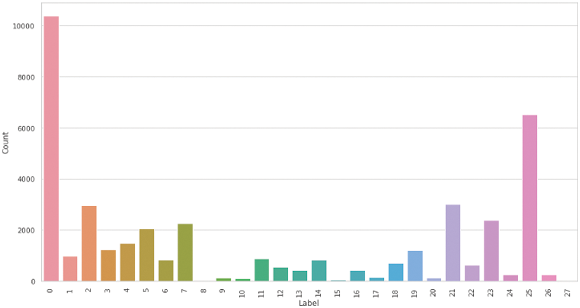
Figure 7: Multiple cells data classes distribution before the balance method

Figure 8: Multiple cells data classes distribution after the balance method

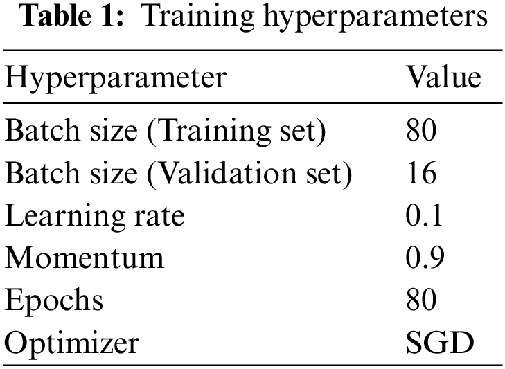
We divided the dataset at the ratio of 80:20 and repeated each experiment using five-fold cross-validation. Table 1 summarizes the chosen values for training hyperparameters, and loss is a binary cross-entropy loss for the multi-label classification task. We used the Stochastic Gradient Descent (SGD) for optimization; it is fast and can converge smoothly. The learning rate is reduced by half when model performance reaches a plateau to achieve the best result.

All model experiments were implemented using TensorFlow. TensorFlow is a machine learning system that runs on several computing devices, including multicore CPUs, general-purpose GPUs, and Tensor Processing Units (TPUs) [37]. TensorFlow covers a wide range of applications, focusing on deep neural network training and inference. The models were trained via Colab Pro + kernels. Technical specifications include a single NVIDIA Tesla P100 GPU with 8 CPU cores and 52 Gigabytes of RAM.

5  Result and Discussion

We have used the GapNet-PL model using PReLU and SeLU activation functions to predict protein localization labels in the multiple cell images dataset. We have evaluated the model performance using 5-fold cross-validation. Table 2 shows the results after calculating the metrics that quantify the model’s performance. Also, we compared the performance of the two activation functions to decide which would give the best results in all performance parameters.

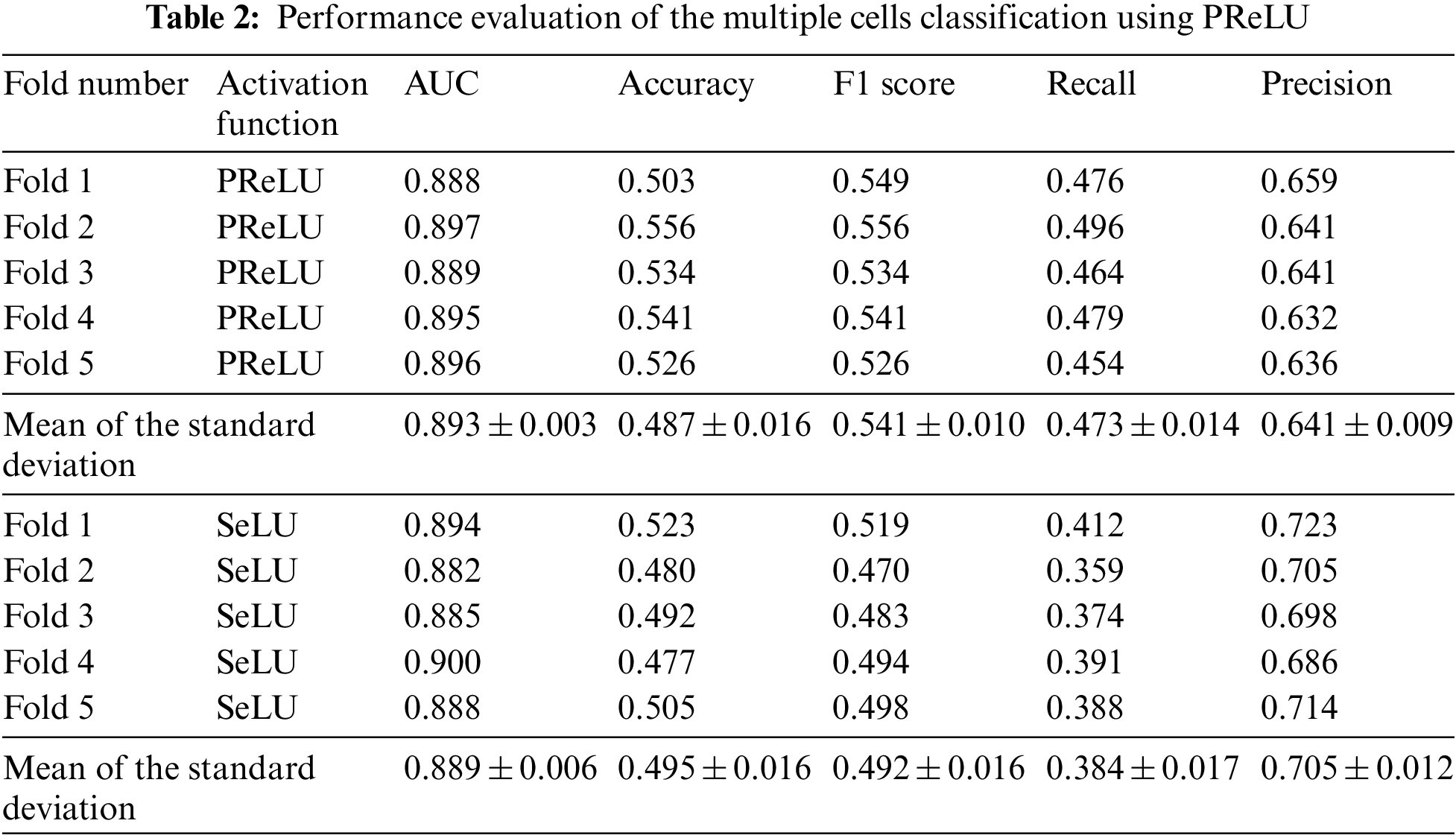
To start with, we obtained good results when we tried the PReLU activation function, as shown in Table 2. The PReLU model surpassed the SeLU model in most metrics. While using the PReLU activation function, the mean of the AUC metric is 0.896, which is 0.4% better than the SeLU activation function. The average classification accuracy for SeLU is 0.495. It outperformed the PReLU model by 1.6%. While the F1 score average is 0.541 for the PReLU model, surpassing the SeLU model by 9.4%. The recall metric’s mean is 0.473, which is better than the SeLU model by 20.7%. Finally, the mean of precision using SeLU is 0.705. It exceeded the mean of PReLU activation by 9.5%. From the previous comparison, we can infer that the PReLU activation function surpassed SeLU activation in three metrics: AUC, F1 score, and Recall. In contrast, SeLU activation outperformed PReLU in the Accuracy and Precision metrics.

Fig. 9 shows the confusion matrix for the PReLU model. We used a library called MLCM (Multi-Label Confusion Matrix) proposed by [38] for defining the confusion matrix for multi-label classifiers. This method presented the multi-class confusion matrix’s well-known structure while meeting the requirements for a 2-dimensional confusion matrix with extra raw and column. The additional column denotes the no predicted labels (NPL), which refers to a circumstance in which there is a combination of true and predicted labels, but no incorrect prediction.

Figure 9: Confusion matrix for GapNet-PL with PReLU

In contrast, one or more true labels are not predicted. The additional row shows the no true labels (NTL), which refers to a circumstance in which there is no true label in the combination of true and predicted labels. The percentage in the diagonal refers to the true classified classes, and the dark colors represent the highest percentage.

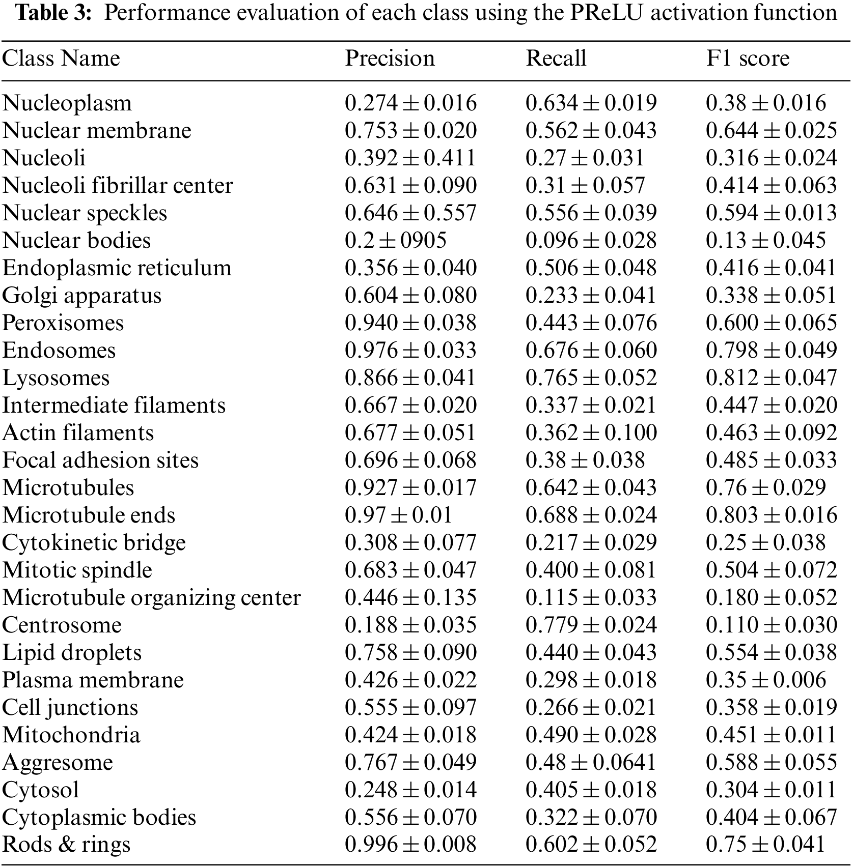
Table 3 summarizes the average of the model’s performance for each class using the PReLU activation function.

Parameter Comparison of True Positive (TP), False Positive (FP), False Negative (FN), and True Negative (TN) for each label in Table 4.

Table 5 compares the performance of the GapNet-PL model using the PReLU activation function with other published results. We can notice that our trained model’s classification accuracy using SeLU and F1 score using PReLU are better than the published results even when using the same data.

6  Conclusion and Future Work

This research uses a deep learning architecture to handle large and complex data. In addition, we use a CNN model called GapNet-PL to classify multi-cell microscopy images into 28 protein classes, while each image can have one or more labels. This study examines another activation function called PReLU and compares it to the SeLU activation function. We applied oversampling and undersampling methods to solve the massive imbalance of data classes. The PReLU model performs perfectly in three metrics, achieving an average AUC of 0.896, an F1 score of 0.541, and a recall of 0.473. The SeLU model performed better in the rest of the metrics and gave an accuracy average of 0.495 and a precision average of 0.705.

F1 score is preferred to be used when there is a significant data imbalance. PReLU outperformed SeLU in F1 score metric, thus we can say that PReLU is better than SeLU in classifying protein images that have imbalanced data distribution. We will try different CNN architectures and other HPA datasets in the future. Moreover, use other activation functions such as Relu and Elu. We also aim to use different sizes of dataset images with different resolutions, as presented in the Kaggle competition.

Acknowledgement: The authors sincerely acknowledge the support from Umm Al-Qura University, Saudi Arabia, for this study.

Funding Statement: The authors received no specific funding for this study.

Conflicts of Interest: The authors declare they have no conflicts of interest to report regarding the present study.

References

1. R. Stadhouders, G. J. Filion and T. Graf, “Transcription factors and 3D genome conformation in cell-fate decisions,” Nature, vol. 569, no. 7756, pp. 345–354, 2019. [Google Scholar] [PubMed]

2. X. Wang, “Human protein classification in microscope images using deep learning and Focal-Lovász loss,” in 2020 4th Int. Conf. on Video and Image Processing, Xi’an, China, pp. 230–235, 2020. [Google Scholar]

3. Y. Shen, Y. Ding, J. Tang, Q. Zou and F. Guo, “Critical evaluation of web-based prediction tools for human protein subcellular localization,” Briefings in Bioinformatics, vol. 21, no. 5, pp. 1628–1640, 2020. [Google Scholar] [PubMed]

4. X. Peng, J. Wang, J. Zhong, J. Luo and Y. Pan, “An efficient method to identify essential proteins for different species by integrating protein subcellular localization information,” in 2015 IEEE Int. Conf. on Bioinformatics and Biomedicine (BIBM), Washington, DC, USA, pp. 277–280, 2015. [Google Scholar]

5. T. Shwetha, S. A. Thomas and V. Kamath, “Hybrid Xception model for human protein atlas image classification,” in Proc. 2019 IEEE 16th India Council Int. Conf. (INDICON), Rajkot, Gujrat, India, pp. 1–4, 2019. [Google Scholar]

6. S. Aggarwal, S. Gupta and R. Ahuja, “A review on protein subcellular localization prediction using microscopic images,” in 2021 6th Int. Conf. on Signal Processing, Computing and Control (ISPCC), Solan, India, pp. 72–77, 2021. [Google Scholar]

7. F. Xing, Y. Xie, H. Su, F. Liu and L. Yang, “Deep learning in microscopy image analysis: A survey,” IEEE Transactions on Neural Networks and Learning Systems, vol. 29, no. 10, pp. 4550–4568, 2017. [Google Scholar]

8. The Human Protein Atlas. Introduction of the human protein atlas, 2003. Available: https://www.proteinatlas.org/about#the_human_protein_atlas [Google Scholar]

9. E. Rumetshofer, M. Hofmarcher, C. Röhrl, S. Hochreiter and G. Klambauer, “Human-level protein localization with convolutional neural networks,” in Proc. Int. Conf. on Learning Representations, New Orleans, USA, pp. 1–18, 2018. [Google Scholar]

10. HPA Team Kaggle. “Human protein atlas image classification,” 2018. Available: https://www.kaggle.com/c/human-protein-atlas-image-classification/data [Google Scholar]

11. W. Ouyang and C. Zimmer, “The imaging tsunami: Computational opportunities and challenges,” Current Opinion in Systems Biology, vol. 4, pp. 105–113, 2017. [Google Scholar]

12. A. Esteva, B. Kuprel, R. A. Novoa, J. Ko, S. M. Swetter et al., “Dermatologist-level classification of skin cancer with deep neural networks,” Nature, vol. 542, no. 7639, pp. 115–118, 2017. [Google Scholar] [PubMed]

13. H. A. Haenssle, C. Fink, R. Schneiderbauer, F. Toberer, T. Buhl et al., “Man against machine: Diagnostic performance of a deep learning convolutional neural network for dermoscopic melanoma recognition in comparison to 58 dermatologists,” Annals of Oncology, vol. 29, no. 8, pp. 1836–1842, 2018. [Google Scholar] [PubMed]

14. D. Devarajan, D. S. Alex, T. Mahesh, V. V. Kumar, R. Aluvalu et al., “Cervical cancer diagnosis using intelligent living behavior of artificial jellyfish optimized with artificial neural network,” IEEE Access, vol. 10, pp. 126957–126968, 2022. [Google Scholar]

15. M. Poostchi, K. Silamut, R. J. Maude, S. Jaeger and G. Thoma, “Image analysis and machine learning for detecting malaria,” Translational Research, vol. 194, pp. 36–55, 2018. [Google Scholar] [PubMed]

16. O. Dürr and B. Sick, “Single-cell phenotype classification using deep convolutional neural networks,” Journal of Biomolecular Screening, vol. 21, no. 9, pp. 998–1003, 2016. [Google Scholar]

17. W. J. Godinez, I. Hossain, S. E. Lazic, J. W. Davies and X. Zhang, “A multi-scale convolutional neural network for phenotyping high-content cellular images,” Bioinformatics, vol. 33, no. 13, pp. 2010–2019, 2017. [Google Scholar] [PubMed]

18. L. Wei, Y. Ding, R. Su, J. Tang and Q. Zou, “Prediction of human protein subcellular localization using deep learning,” Journal of Parallel and Distributed Computing, vol. 117, pp. 212–217, 2018. [Google Scholar]

19. J. X. Hu, Y. Y. Xu and H. B. Shen, “Deep learning-based classification of protein subcellular localization from immunohistochemistry images,” in Proc. 2017 4th IAPR Asian Conf. on Pattern Recognition (ACPR), Nanjing, China, pp. 599–604, 2017. [Google Scholar]

20. O. Z. Kraus, B. T. Grys, J. Ba, Y. Chong, B. J. Frey et al., “Automated analysis of high-content microscopy data with deep learning,” Molecular Systems Biology, vol. 13, no. 4, pp. 1–15, 2017. [Google Scholar]

21. E. Zhang, B. Zhang, S. Hu, F. Zhang, Z. Liu et al., “Multi-labelled proteins recognition for high-throughput microscopy images using deep convolutional neural networks,” BMC Bioinformatics, vol. 22, no. 3, pp. 1–15, 2021. [Google Scholar]

22. A. Mitra, “Multi-label classification of human protein subcellular locations from microscopy images using convolutional neural networks,” Masters Thesis, Bangladesh University of Engineering and Technology, Bangladesh, 2021. [Google Scholar]

23. D. P. Sullivan, C. F. Winsnes, L. Åkesson, M. Hjelmare, M. Wiking et al., “Deep learning is combined with massive-scale citizen science to improve large-scale image classification,” Nature Biotechnology, vol. 36,no. 9, pp. 820–828, 2018. [Google Scholar] [PubMed]

24. K. Liimatainen, R. Huttunen, L. Latonen and P. Ruusuvuori, “Convolutional neural network-based artificial intelligence for classification of protein localization patterns,” Biomolecules, vol. 11, no. 2, pp. 1–15, 2021. [Google Scholar]

25. H. Y. Chang and C. L. Wu, “Deep learning method to classification human protein Atlas,” in Proc. 2019 IEEE Int. Conf. on Consumer Electronics-Taiwan (ICCE-TW), Yilan, Taiwan, pp. 1–2, 2019. [Google Scholar]

26. Y. Tu, H. Lei, H. B. Shen and Y. Yang, “SIFLoc: A self-supervised pre-training method for enhancing the recognition of protein subcellular localization in immunofluorescence microscopic images,” Briefings in Bioinformatics, vol. 23, no. 2, 2022. https://doi.org/10.1093/bib/bbab605 [Google Scholar] [PubMed] [CrossRef]

27. P. Rana, A. Sowmya, E. Meijering and Y. Song, “Imbalanced classification for protein subcellular localization with multilabel oversampling,” Bioinformatics, vol. 39, no. 1, 2023. https://doi.org/10.1093/bioinformatics/btac841 [Google Scholar] [PubMed] [CrossRef]

28. T. Jiang and J. Cheng, “Target recognition based on CNN with LeakyReLU and PReLU activation functions,” in Proc. 2019 Int. Conf. on Sensing, Diagnostics, Prognostics, and Control (SDPC), Beijing, China, pp. 718–722, 2019. [Google Scholar]

29. K. M. A. Adweb, N. Cavus and B. Sekeroglu, “Cervical cancer diagnosis using very deep networks over different activation functions,” IEEE Access, vol. 9, pp. 46612–46625, 2021. [Google Scholar]

30. K. Shridhar, J. Lee, H. Hayashi, P. Mehta, B. K. Iwana et al., “Probact: A probabilistic activation function for deep neural networks,” arXiv:1905.10761v2, pp. 1–14, 2019. https://doi.org/10.48550/arXiv.1905.10761 [Google Scholar] [CrossRef]

31. H. X. Guo, Y. J. Li, J. Shang, M. Y. Gu, Y. Y. Huang et al., “Learning from class-imbalanced data: Review of methods and applications,” Expert Systems with Applications, vol. 73, pp. 220–239, 2017. [Google Scholar]

32. N. V. Chawla, K. W. Bowyer, L. O. Hall and W. P. Kegelmeyer, “SMOTE: Synthetic minority over-sampling technique,” Journal of Artificial Intelligence Research, vol. 16, pp. 321–357, 2002. [Google Scholar]

33. M. A. Tahir, J. Kittler, K. Mikolajczyk and F. Yan, “A multiple expert approach to the class imbalance problem using inverse random under sampling,” in Proc. Multiple Classifier Systems, Reykjavik, Iceland, pp. 82–91, 2009. [Google Scholar]

34. U. Batool, M. I. Shapiai, N. Ismail, H. Fauzi and S. Salleh, “Oversampling based on data augmentation in convolutional neural network for silicon wafer defect classification,” in Proc. 19th Int. Conf. on New Trends in Intelligent Software Methodologies, Tools and Techniques (SoMeT_20), Amsterdam, The Netherlands, vol. 327, pp. 3–12, 2020. [Google Scholar]

35. K. He, X. Zhang, S. Ren and J. Sun, “Delving deep into rectifiers: Surpassing human-level performance on imagenet classification,” in Proc. IEEE Int. Conf. on Computer Vision, Cambridge, MA, USA, pp. 1026–1034, 2015. [Google Scholar]

36. S. Narkhede. “Understanding AUC-ROC curve,” 2018. Available: https://towardsdatascience.com/understanding-auc-roc-curve-68b2303cc9c5 [Google Scholar]

37. M. Abadi, P. Barham, J. Chen, Z. Chen, A. Davis et al., “TensorFlow: A system for large-scale machine learning,” in Proc. 12th USENIX Symp. on Operating Systems Design and Implementation (OSDI’ 16), Savannah, GA, USA, pp. 265–283, 2016. [Google Scholar]

38. M. Heydarian, T. E. Doyle and R. Samavi, “MLCM: Multi-label confusion matrix,” IEEE Access, vol. 10, pp. 19083–19095, 2022. [Google Scholar]