An Improved Deep Structure for Accurately Brain Tumor Recognition

1  Introduction

Brain neoplasms, also known as intracranial tumors, are more commonly affected in all human age classes, older adults, toddlers, and infants. Carcinogenic factors, such as ionizing radiation and the family history of the disease, are two of the most common brain cancer causes [1]. The major problem of brain cancer is the lack of control growth of normal cells, which causes an esteemed uncontrolled growth of tumors, disrupting normal tissues and causing shear stress on cells, eventually killing them. Early diagnosis is critical for reducing long-term morbidity and mortality rates by reducing life-threatening cancer disease complications and saving appropriate treatment on time [1]. Accordingly, the need for an automatic, quick, and accurate brain tumor recognition algorithm considers essential. There are several methods of tumor imagining scans, such as magnetic resonance imaging (MRI) [2], computed tomography (CT) [3], positron emission tomography (PET) [4], single photon emission computed tomography (SPECT) scans [5], and cerebral angiography [6].

The most common technique is MRI, which has the following advantages: nonionizing, reducing the risk of harm to healthy tissues, generating 3-D images efficiently, and precise localization of the brain tumor. The main aim of this study is to identify and recognize brain tumors using a deep learning structure and exclude them from the other tissues such as grey and white brain matter, and cerebrospinal fluid (CSF).

The major contributions of this study are:

     i)  Extracting low levels of salient features from the GLCM data frame, including energy, correlation, contrast, homogeneity, and dissimilarity, then selecting the best of them using a proposed DNN model.

    ii)  Extracting a high level of salient features from a proposed CNN deep structure with a robust layering structure and fine-tuned hyperparameters.

   iii)  Concatenating the two types of extracted features to form a homogenous features data frame.

    iv)  Proposing an additional DNN model that fed with the homogenous features matrix as an input layer to additional deep layers which directly increases the recognition accuracy in both single and multi-classes of datasets.

The rest of this manuscript is summarized as follows: Section 2 introduces the recent related works, Section 3 presents the principal methodology of the proposed fused algorithm, Section 4 shows the experimental results of this study and its discussions, and finally, the conclusions and the expected future works.

2  Related Works

Vankdothu et al. proposed a model that detects and classifies brain tumor grades, including glioma, meningioma, pituitary tumor, and no tumor. They combined a CNN with a Long Short-Term Memory (STM) to extract the main brain features. Finally, the images have been classified and scored 89.39% accuracy in CNN, 90.02% in recurrent neural network (RNN), and 92% in the CNN-LSTM method [7].

Srikanth et al. introduced computer-assisted technology to detect and diagnose brain tumor disease automatically. Instead of using traditional machine learning algorithms (ML), they proposed a deep neural network based on the Visual Geometry Group (VGG-16) to improve the multi-classification accuracy value. Extensive experiments demonstrate that the updated VGG-16 model outperforms the current studies in terms of performance metrics [8].

Deshpande et al. proposed a fused algorithm to recognize a brain tumor based on a deep learning structure. Their framework has been merged with a Discrete Cosine Transform (DCT), CNN, and ResNet50 into one model to improve the recognition accuracy. The experimental results reveal that the proposed model scores the best in evaluating metrics [9].

Abirami et al. proposed a model called Border Collie Firefly Algorithm-based Generative Adversarial Network (BCFA-based GAN), which classifies the severity level of brain tumors effectively. They preprocessed the brain images using a Laplacian filter and then segmented them by a deep joint model. Furthermore, the main features have been extracted, including statistical and Texton and Karhunen-Loeve Transform-based features using slave nodes. Finally, the extracted features were classified using BCFA-based GAN and scored 97.515% of classification accuracy [10].

An adaptive multisequence fusing neural network (AMF-Net) has been implemented by Huang et al. to precisely diagnose brain tumor grades. This model can merge the different MRI characteristics of sequences with adaptive weights. The experimental results score the accuracy value ranged between 92.1% and 98.1% [11].

Irmak presented the three different CNN models to improve the detection of a brain tumor automatically and accurately. The second CNN splits the database into five brain tumor categories: normal, glioma, meningioma, pituitary, and metastatic. Moreover, the third CNN divides brain tumors into three grades: Grade II, Grade III, and Grade IV scoring 92.66% and 98.14% classification accuracy, respectively, when the hyperparameters are tuned using a grid search optimization algorithm. Finally, to confirm the robustness of the proposed model, its experimental results have been compared with the pre-trained models such as ResNet-50, Alex Net, Inceptionv3, VGG-16, and GoogleNet and scored the best performance metrics values [12].

Chanu et al. differentiate between benign and malignant tumors using the computer-aided algorithm based on a 2D convolutional neural network model. The proposed model can classify MRI images as normal and tumor classes with 97% classification accuracy [13].

In [14], Zeineldin et al. presented a brain tumor segmentation model named DeepSeg, which divides each MRI image into two corresponding core parts based on the relation between encoding and decoding algorithms. A convolutional neural network (CNN) is used as an encoder to extract spatial information. Then, the resulting semantic map is used as the decoder part for getting a high-resolution probability map based on modified U-Net architecture. Different CNN models have also been utilized, such as residual neural networks (ResNet), dense convolutional networks (DenseNet), and NASNet.

In [15], the brain tumor features have been extracted from MR images using the pre-trained models, Dense+Net-41, and ResNet-50. Afterward, the extracted features have been localized and classified using the proposed model, called a custom Mask Region-based Convolution neural network (Mask RCNN). This work achieved the best performance compared to the recent state-of-the-art studies.

3  Framework for Brain Tumor Recognition

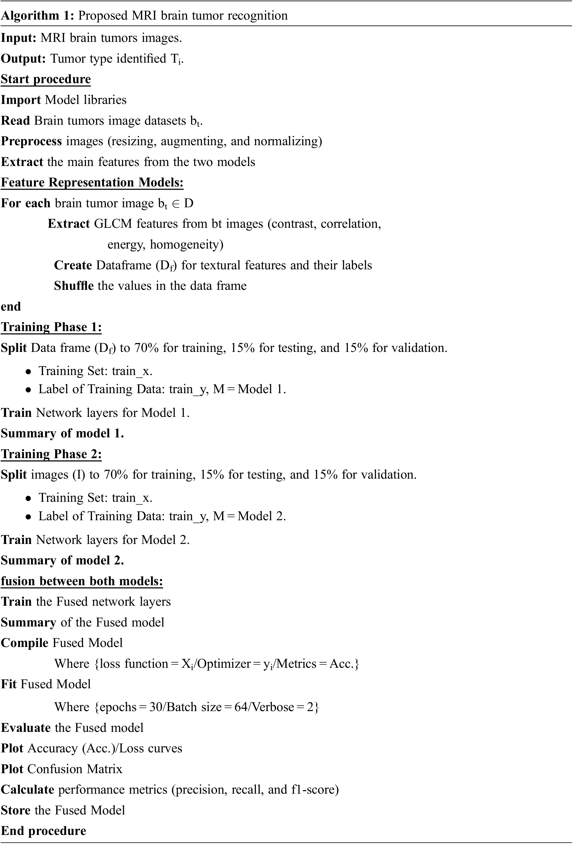
Fig. 1 shows the main components of the proposed brain tumor recognition algorithm. Fig. 2 refers to the block diagram of the proposed methodology that starts by loading and extracting images and their labels from different datasets and then applying preprocessing and augmentation techniques. After that, splitting the dataset to train, test, and validate categories.

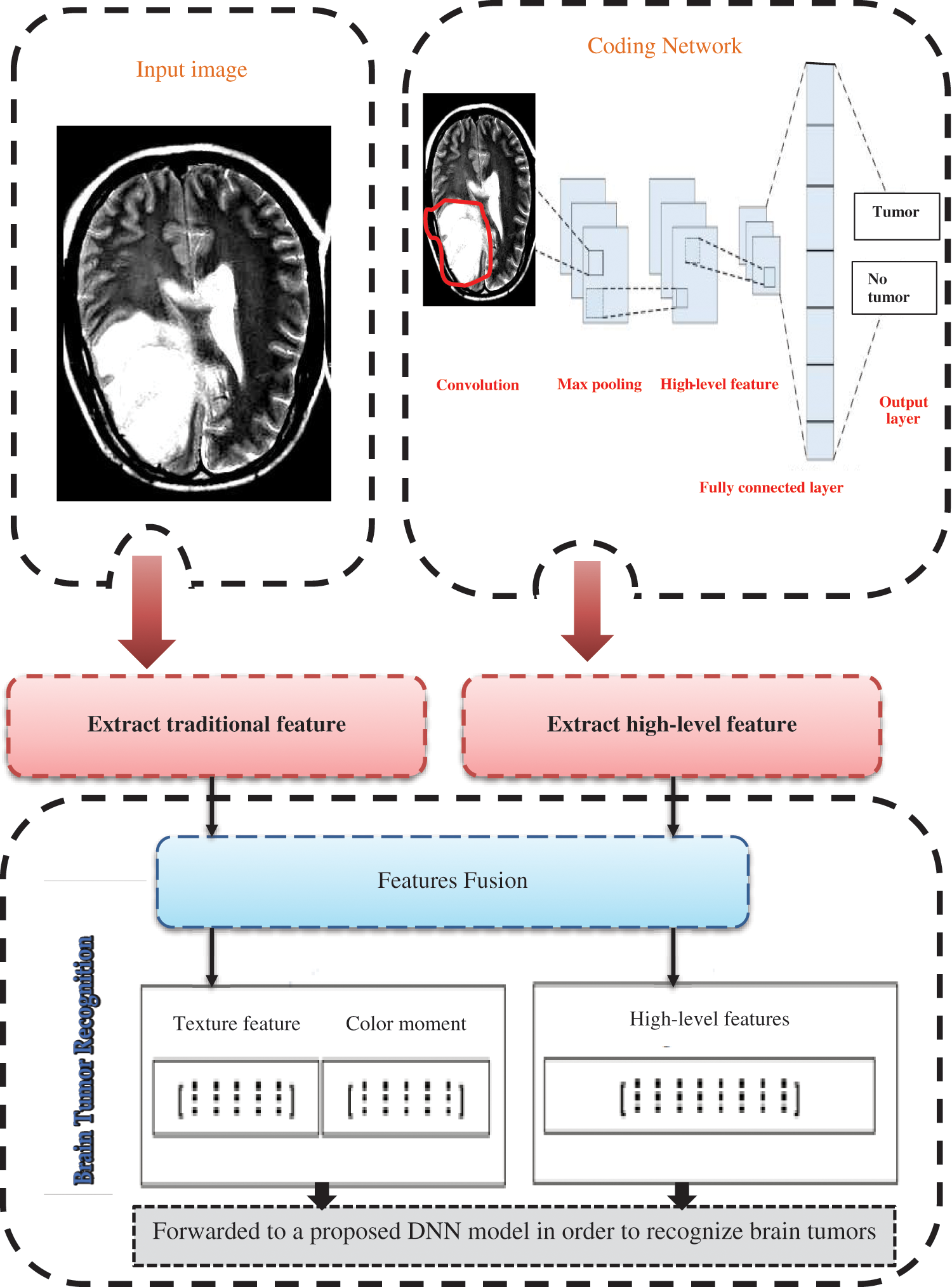
Figure 1: Introduces the proposed brain tumor recognition methodology

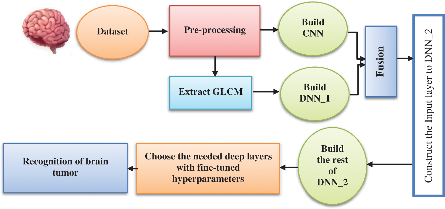
Figure 2: Block diagram of the proposed deep structure

3.1 Datasets

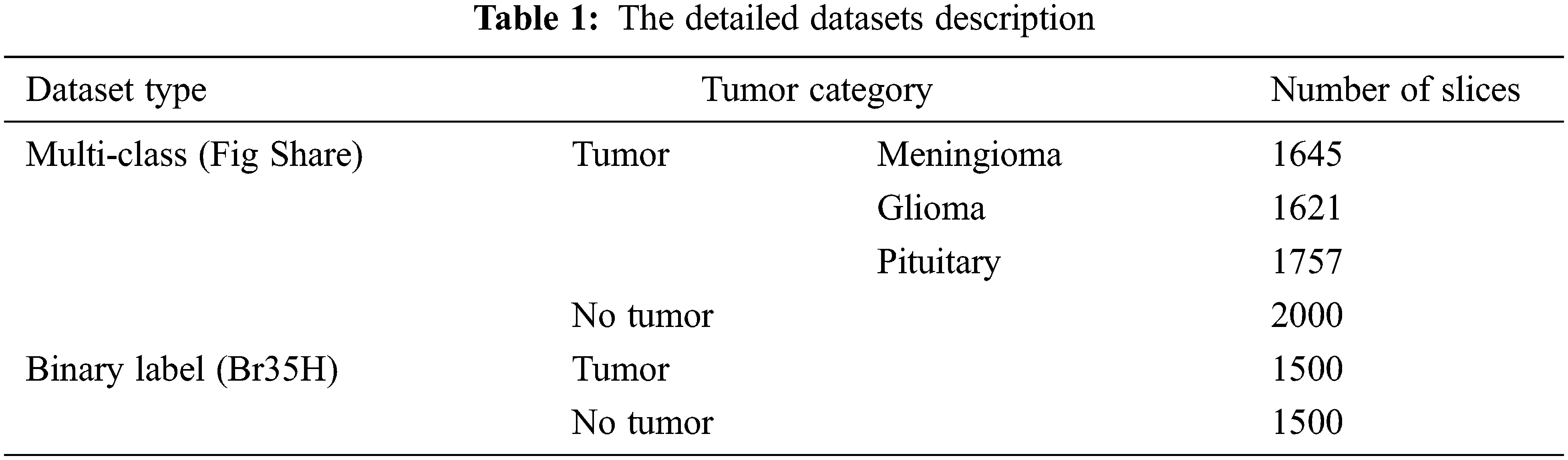
The presented study has been built based on two standard MRI datasets, a multi-class dataset and a binary one. The first dataset captures from Nanfang Hospital and General Hospital, Tianjin 107 Medical University, China, between 2005 and 2007. It was published online in 2015 [16], and the most recent 108 revisions were completed in 2017. This dataset contains three different cases of brain tumors, including (meningioma, glioma, and pituitary) and no tumors. All MRI images have been acquired from three different views: axial (994 images), coronal (1045 images), and sagittal (1025 images) views [17]. On the other side, the second dataset can distinguish between equally healthy and tumor cases to form a 3000 MRI images dataset [18]. Fig. 3 refers to the sample of the different applied datasets, and the detailed datasets have been tabulated in Table 1.

Figure 3: Sample of both Datasets (a) Multi-class MRI and (b) Binary MRI

3.2 Preprocessing Stage

Firstly, the image size has been decreased to 140 × 140 × 1 to reduce dimensionality which has a great impact on the training time. Moreover, splitting the image datasets into the train, test, and validation sets with the percentage of (70% for training, 15% for testing, and 15% for the validation process). Accordingly, shuffling and normalizing datasets have been performed according to Eq. (1) [19],

 A^=(A−min valueofAmax value of A−minvalueofA)∗(R−M)+M  (1)

where A^ is Min-Max Normalized data, R and M are the predefined boundaries, and the range of the original data is A.

Finally, some geometric augmentation processes on split images, including right/left mirror, flipping them around the x-axis. Fig. 4 refers to the main used augmentation process.

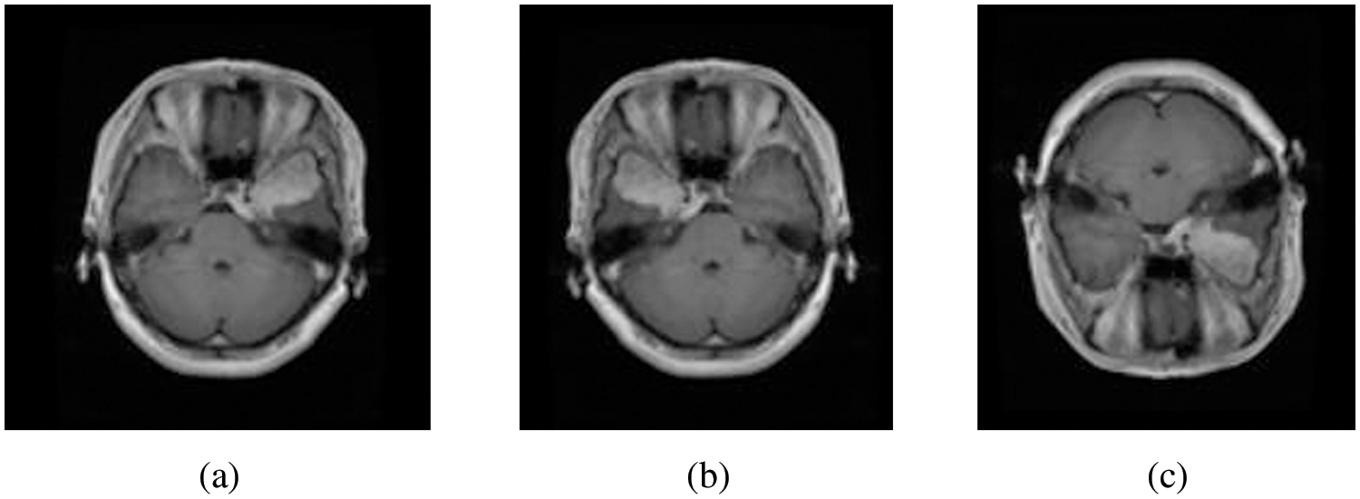
Figure 4: (a) Original image, (b) right/left mirror, and (c) up/down flipping

3.3 Feature Representation Methods

This section describes the proposed feature extraction criteria for the process of brain tumor recognition. The textural features selected for the first model and Gray Level Co-occurrence Matrix (GLCM), are spatial features extracted from the co-occurrence matrix [20]. Four main texture features have been selected, including contrast, correlation, energy, and homogeneity [21]. The contrast is also called the sum of squares variance, which displays the difference between co-occurrence pairs of pixels over the entire data image and computes by Eq. (2) [22],

Contrast=∑i∑j(i−j)2 p(i, j)   (2)

where p (i, j) refers to the probability of pair of image pixels having gray level values i and j appearing at a given space and direction.

The correlation computes the gray-level linear dependence between pixels at given spaces from each other, which formulates by Eq. (3), where μi and μj are the mean of every row and column, and σi and σj are the standard deviations of every row and column, respectively.

Correlation=∑i∑jp(i, j)[(i−μi)(j−μj)]σiσj  (3)

Energy, known as angular second moment (ASM), refers to the degree of homogeneity of the gray level distribution and the thickness of texture, which measures the greyscale patterns, thus obtaining a significant value of the energy feature needs a more stable regulation. Moreover, the energy is the quadratic sum of GLCM elements and measures the concentration of the gray level intensity according to Eq. (4) [23],

ASM=∑i⁡∑j⁡P (i, j)2  (4)

Homogeneity refers to the structural similarity of an image, which computes by Eq. (5) [24],

Homogeneity=∑i⁡∑jp(i, j)1+|i−j| (5)

Finally, after the GLCM features have been extracted, the data frames now have been formulated and used as input for the proposed deep structure to select the best of them. Fig. 5 introduces a sample of the GLCM Data frame.

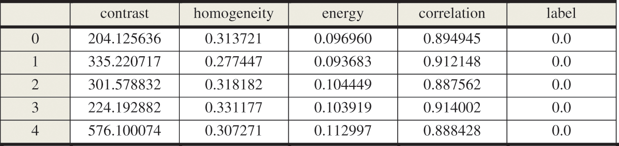
Figure 5: Sample of GLCM data frame

The second model was created based on the proposed CNN architecture to extract the main features from the enhanced MRI brain image datasets. It contains three convolutional layers that use the convolution kernel to extract the best feature information from the input matrix with the ReLU activation function defined in Eq. (6) [25]. Moreover, two max-pooling layers with size (2 × 2) downsampling the input matrix by replacing the pooling area with its maximum value to speed up the training efficiency while retaining meaningful information, which defines by Eq. (7) [26],

f(x)ReLU=max(0, x) (6)

pu,vmax=i,j∈yu,vmaxai,j  (7)

The dropout layer is also added to reduce overfitting, which may occur during the training process, and flattens the neurons at the end; Fig. 6 shows the proposed CNN structure. Finally, after building both feature extraction models, the concatenation fusion was applied between them, which formulates in Eq. (8) [27]. The fully connected layer has been added and followed by a SoftMax layer with two neurons output in the case of a binary dataset and repeated with four neurons output in a multi-class dataset, computed by Eq. (9) [28].

RF=max(0, ∑inwili+∑imwjhj+b) (8)

where Ph1_F =   {l1, l2, l3, l4, …, li, …, ln} , and Ph2_F =  {h1, h2, h3, h4, …, hj, …, hm} represent model one, model two features, and b is the model bias.

sm(z)i= ezi∑j=1k⁡ezj for i=1, …, k and z=(z1, …,  zk)∈Rk  (9)

where zi refers to the element number, z is the input vector, and the resulting values have normalized by dividing the sum of all the exponentials. Algorithm 1 describes the proposed brain tumor recognition, Fig. 7 describes the detailed layer of the proposed model, and Fig. 8 shows its main architecture. Both Figs. 7, and 8 represent the main deep layering structure in the case of using multi-class datasets of output = 4 classes. However, in the case of using any binary dataset with output = 2 classes, the output layer will be altered to be 2 outputs only.

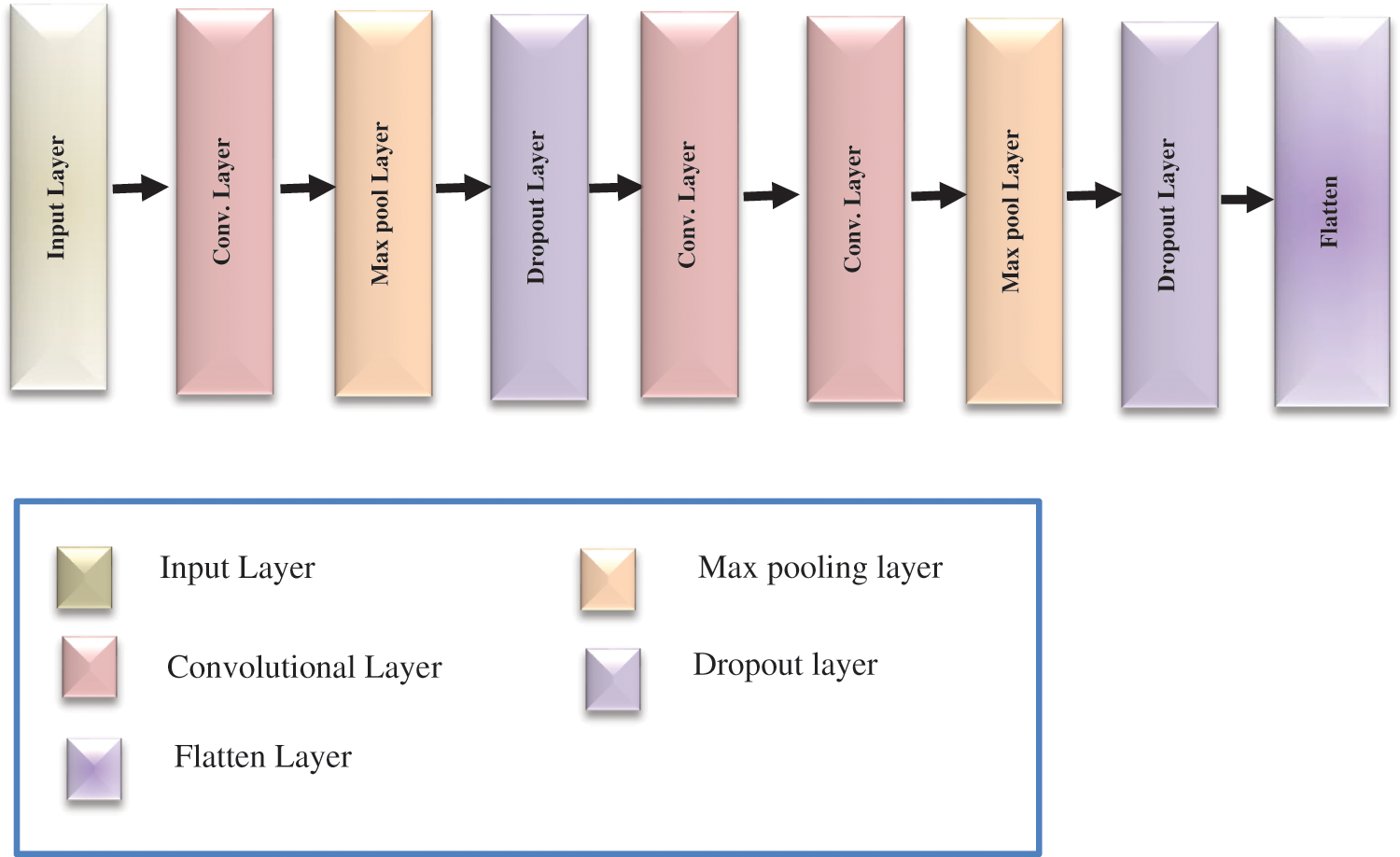
Figure 6: The proposed CNN architecture

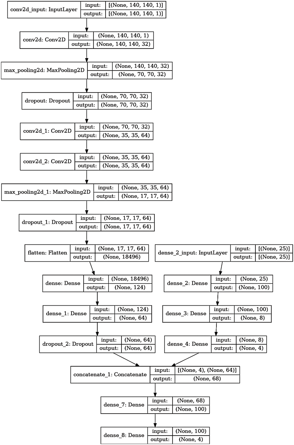
Figure 7: The detailed layers of the proposed multi-class model

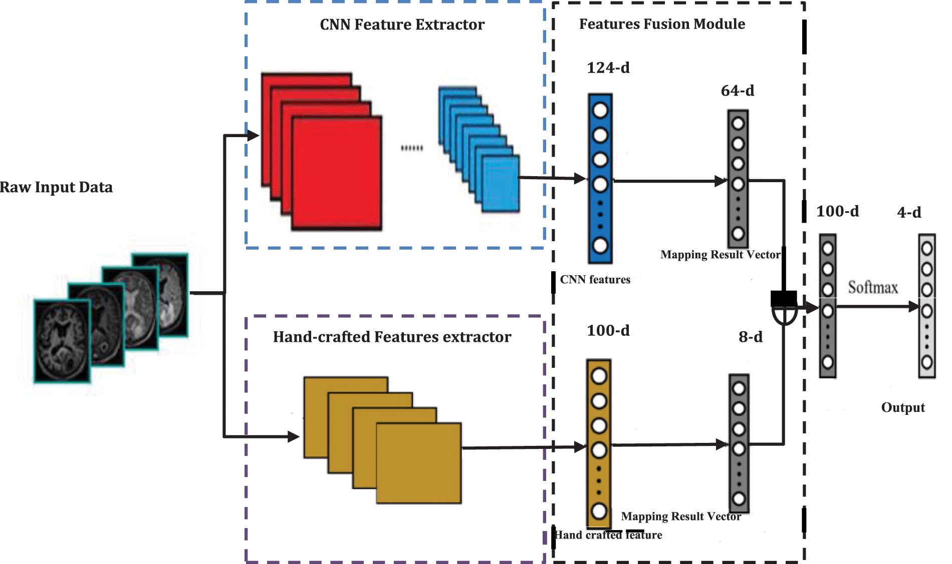
Figure 8: The main architecture of the proposed four classes recognition model

4  Results and Discussions

For evaluating the proposed model results, there are several parameters that must be extracted from the confusion matrix first, including true positive (TP), true negative (TN), false positive (FP), and false negative (FN). Figs. 9 and 10 show the resulting confusion matrix from both multi-class and binary datasets. Eight performance metrics have been computed from these parameters: accuracy, sensitivity, specificity, precision, false discovery rate, F1-score, training time, and recall. The accuracy of the fused model computed from Eq. (10) [29],

Accuracy=TP+TNTP+TN+FP+FN×100 (10)

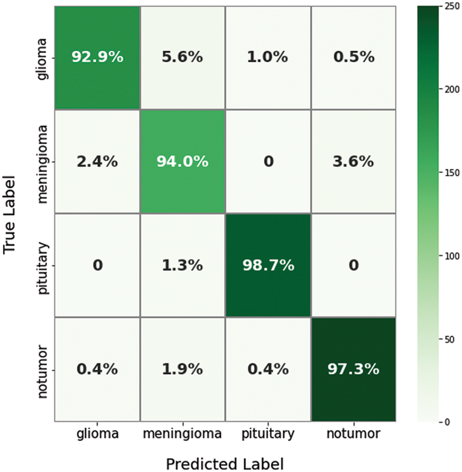
Figure 9: The confusion matrix of the proposed model for a multi-class dataset

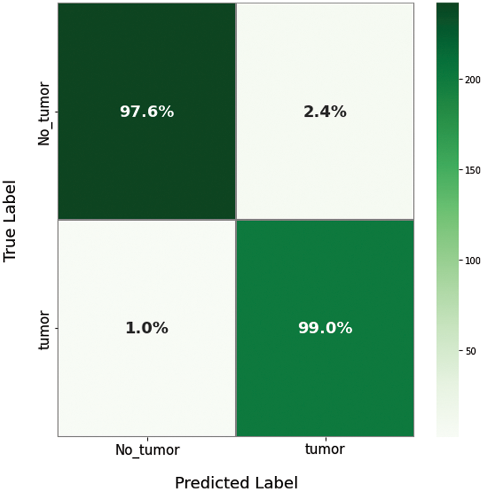
Figure 10: The confusion matrix of the proposed model for a binary dataset

Sensitivity or a true positive rate (TPR), which can measure the correctly recognized sets from a dataset and computes from Eq. (11) [30],

TPR=TPTP+FN×100 (11)

The specificity is, also called True Negative Rate (TNR), can measure the not correctly learned samples from a dataset, which computed from Eq. (12) [30],

TNR=TNTN+Fp×100 (12)

The number of accurately predicted data that turned out to be positive is precision, which calculates from Eq. (13) [31],

PPV=TPTP+FP×100 (13)

F1-score refers to the weighted average of precision and recall computed from Eq. (14) [32],

F1−score=2TP2TP+FP+FN×100 (14)

The False Discovery Rate (FDR) is a metric that estimates the irrelevant alerts, as calculated by Eq. (15) and the False Negative Rate (FNR) obtained from Eq. (16) [33],

FDR=FPFP+TP×100 (15)

FNR=FNFN+TP×100 (16)

where TP is a true positive value, TN is a true negative value, FP is a false positive value, and FN is the false negative value.

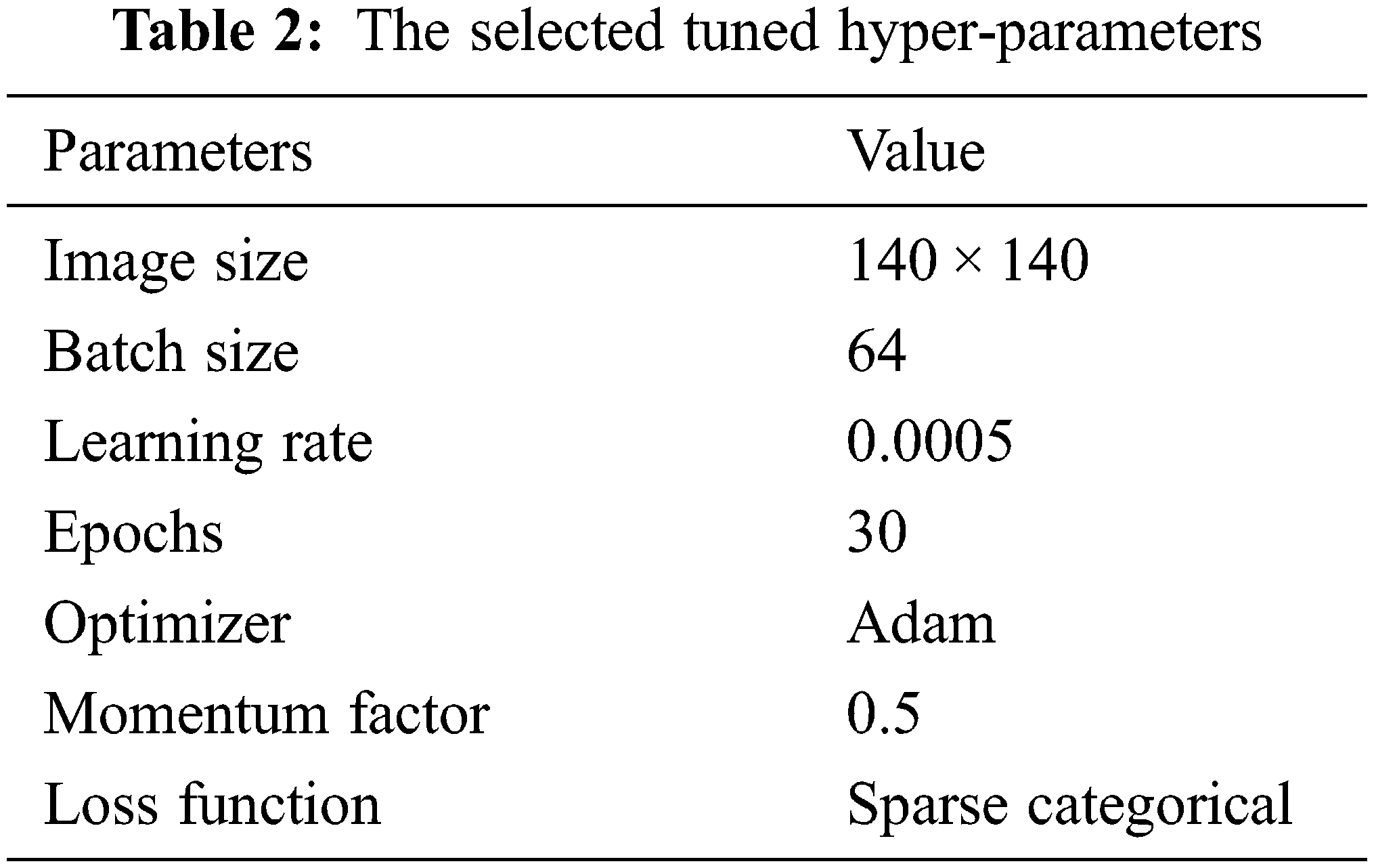
The dataset has been split first to train, test, and validate with a 70%:15%:15% ratio to evaluate the mentioned performance metrics. Then, compiling and fitting the proposed model according to the number of the selected tuned hyperparameters, including batch normalization, reduces the value of the internal shift of the activation layers with size 64. The parameters update step size or learning rate with a value of 0.0005, the sparse categorical cross-entropy for the loss function [33], and the momentum factor value sets to 0.5. Moreover, to consume less memory size and computational time, the Adam optimizer selects for training the proposed fused mode. The main hyper-parameters applied in the proposed models in this manuscript have been tabulated in Table 2. The proposed models have been programmed and tested on a PC having these specifications: Microsoft Windows 10 operating system, 7-core processor @ 4.0 GHz, 12 GB of RAM, NVidia Tesla 16 GB GPU.

4.1 Evaluation of Binary Dataset (Br35H)

According to the appropriate tuning parameters listed in Table 2, the proposed fusion model has been assessed using the binary dataset, which contains two classes: brain tumor and no tumor. The evaluation metrics of the proposed model from the binary dataset have been extracted from its confusion matrix parameters, including a true positive value, a true negative value with the same value of 221, a false positive value, and a false negative value with an equal value of 4. Accordingly, the mentioned equations of the performance metrics have been computed using these parameters and listed in Table 3. In addition, Figs. 11 and 12 show the loss and accuracy curves of the proposed model and the precision-recall curves, respectively, which scored 98.22% of accuracy in a total training time of nearly 30 s.

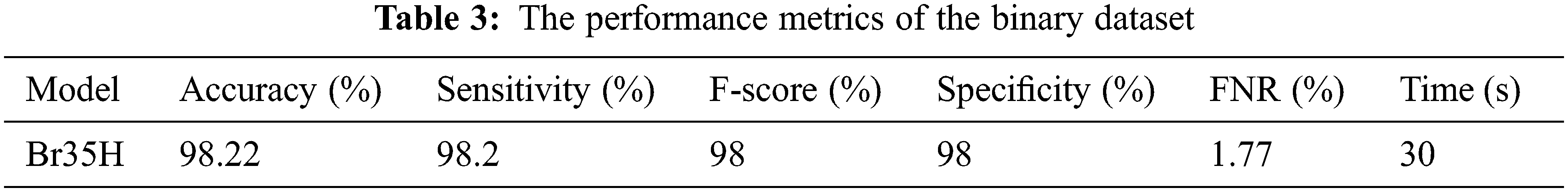
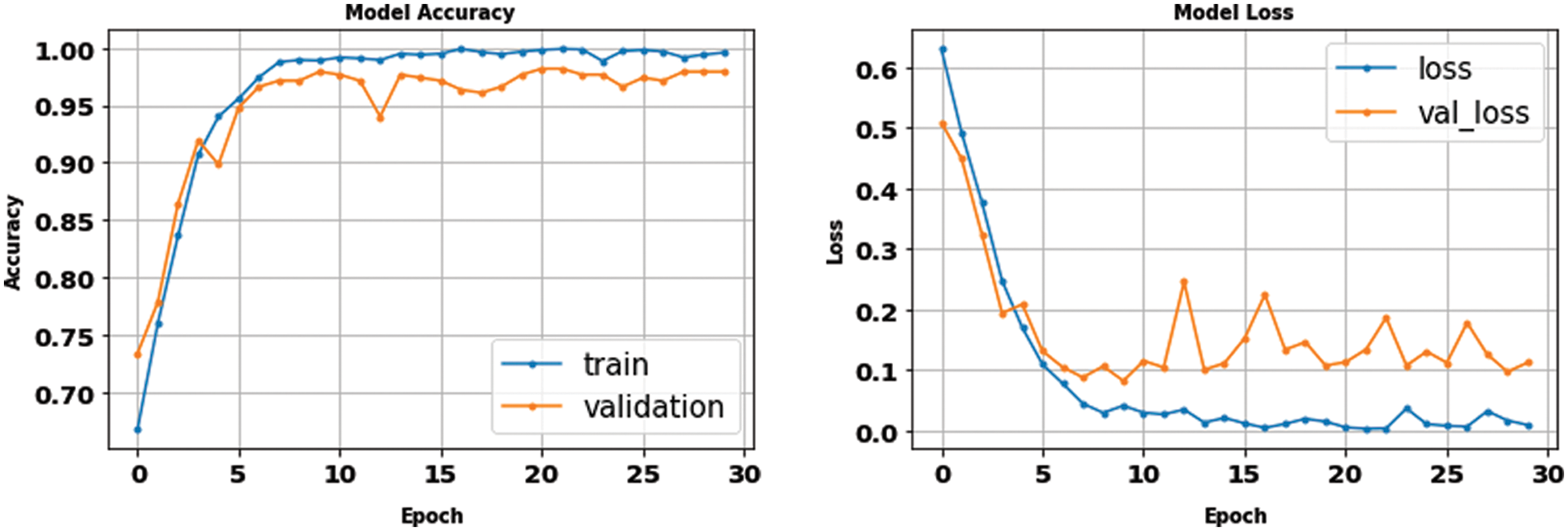
Figure 11: The accuracy and loss curves of the binary dataset with fusion

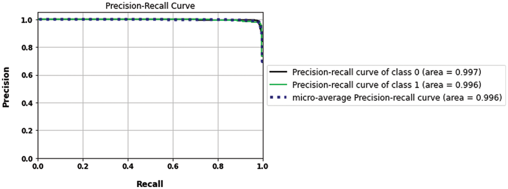
Figure 12: The precision-recall curves of the binary dataset

4.2 Evaluation of Multi-Class Dataset (Fig Share)

Moreover, the proposed methodology has been applied and tested using the multi-class dataset (Fig Share) with the same optimum tuning parameters listed in Table 2. The main parameters of the multi-class model have been extracted from its confusion matrix in Fig. 9, which reached 98.01% accuracy in a training time of nearly 50 s, and then tabulated with the other performance metrics in Table 4. Furthermore, Table 5 shows the detailed accuracy of each class, including Meningioma, Glioma, Pituitary, and no tumor, and Figs. 13 and 14 show the accuracy and loss curves and precision-recall curves, respectively.

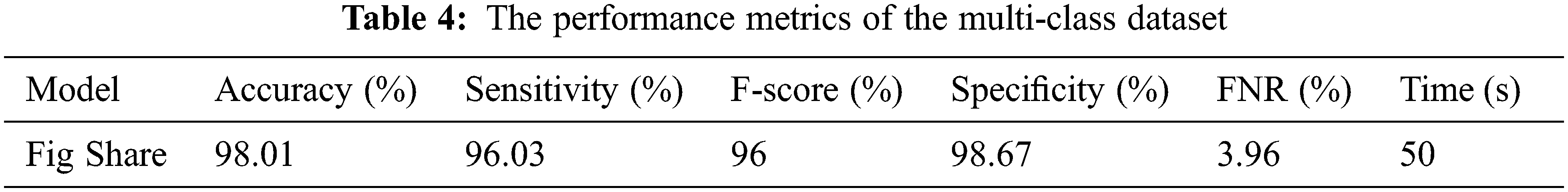
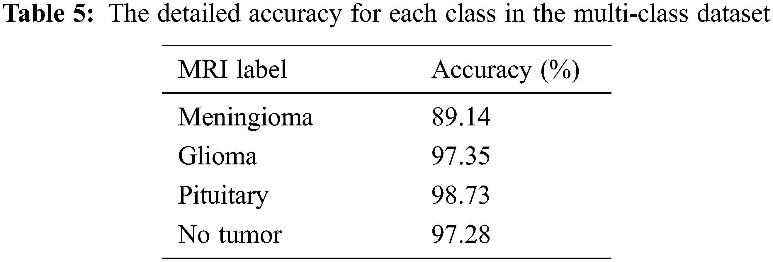
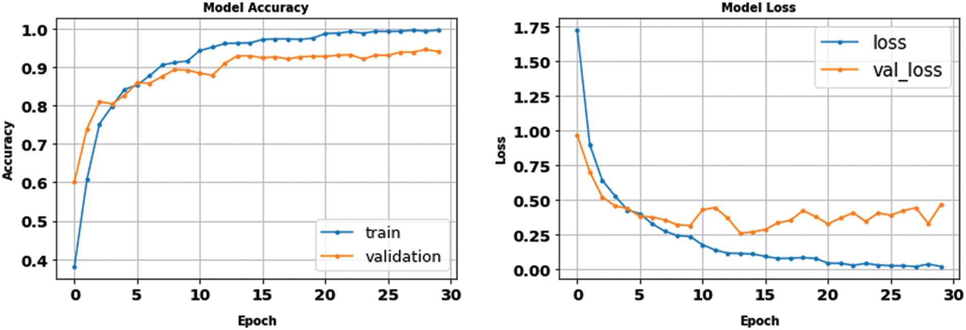
Figure 13: The accuracy and loss curves of the multi-class dataset with fusion

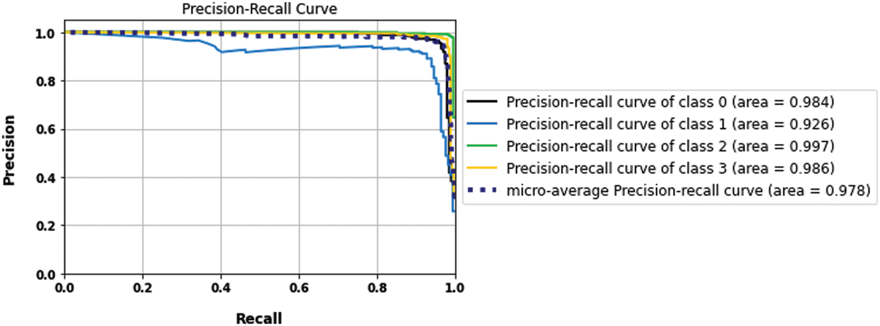
Figure 14: The precision-recall curves of the multi-class dataset

The proposed model results with binary and multilabel datasets had compared to the same CNN architecture but without fusion with GLCM and scored 97.5% and 97.02% in accuracy value, respectively. Fig. 15. shows the loss and accuracy curves of the binary and multilabel datasets of the CNN model, and Fig. 16. shows the output detection of both datasets. Moreover, Fig. 17 shows the precision-recall curves, and Table 6. lists the main performance results of all proposed models and the best one.

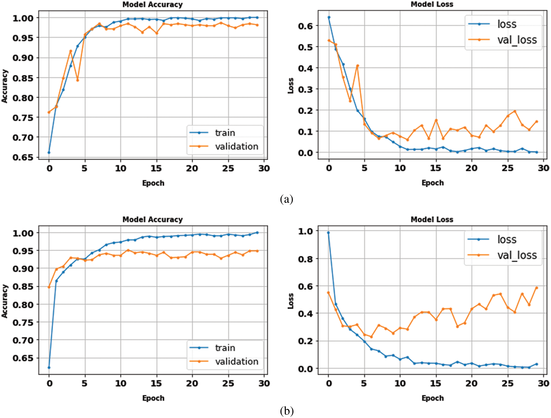
Figure 15: The accuracy and loss curves of CNN models (a) binary dataset, (b) the multi-class dataset without fusion

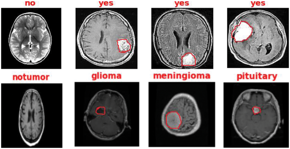
Figure 16: The output detection of binary and multi-class datasets

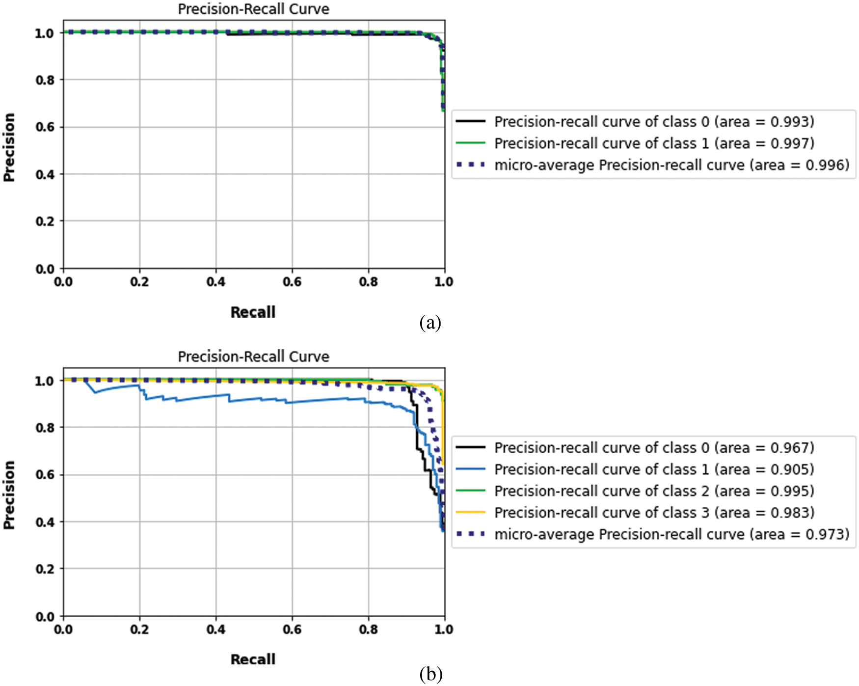
Figure 17: The precision and recall curves of CNN models (a) binary dataset, (b) the multi-class datasets

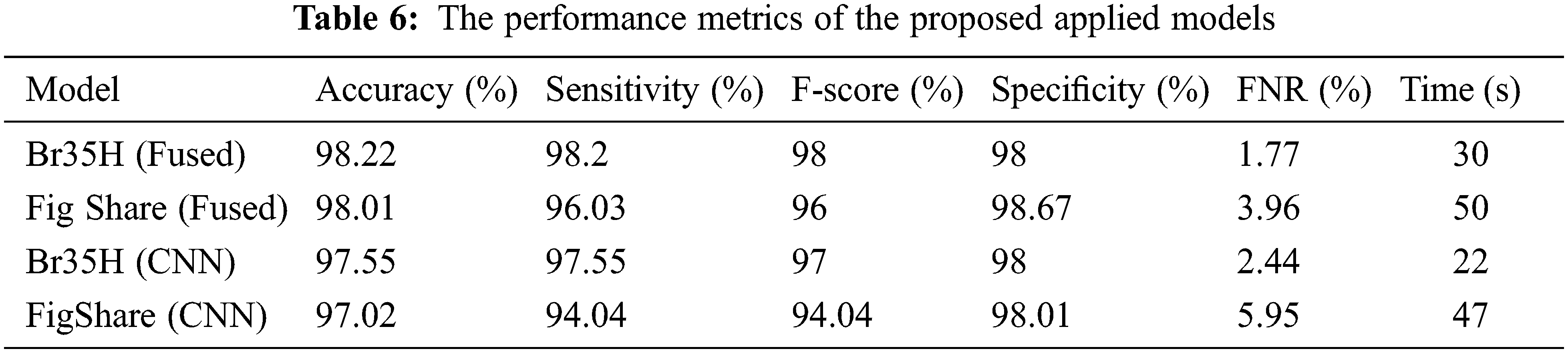
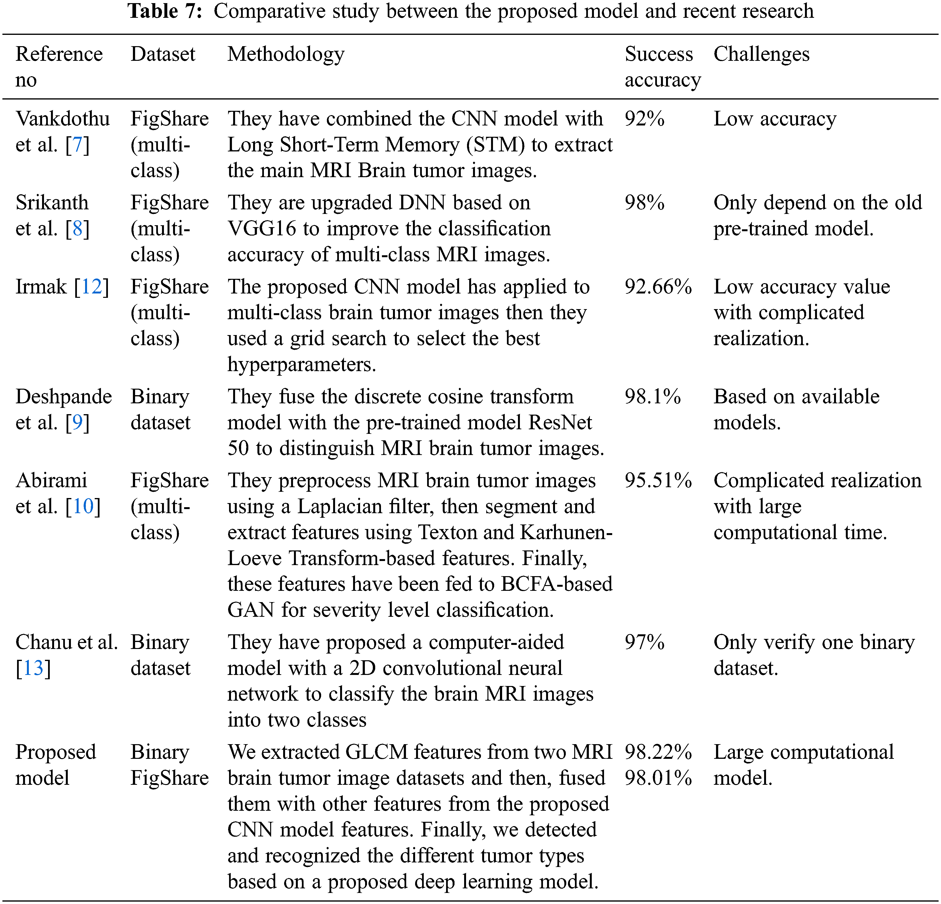
Finally, the proposed models also have been compared with recent research in [7,8,10,12], then tabulated these results in Table 7. The proposed model results in the mentioned table scored 98.22% in recognition accuracy value in the low training time, enhancing the brain tumor’s detection and recognition and outperforming the current state-of-the-art studies.

5  Conclusion

This paper proposes a CNN and GLCM feature fusion recognition technique to detect and recognize MRI brain tumor images into four classes. MRI images have been preprocessed, segmented, enhanced, and tested using a robust DNN architecture. According to the appropriate evaluation metrics, a comprehensive study has been manipulated between the proposed methodology and the current state-of-the-art to ensure the robustness of the proposed model. Experimental recognition results have proved that the performance of the proposed fusion model outperforms any of the recent techniques in state of art of accuracy, sensitivity, specificity, FNR, recall, and training time. The proposed fusion model scores about 98.22% and 98.01% on both binary and multi-class dataset’s accuracy values respectively. Furthermore, it scored about 98.2%, 98%, and 1.77% in sensitivity, specificity, and FNR, respectively, within 30 s only. Future work of interest will be targeting the fusion between other feature extractors in state of art of deep learning.

Acknowledgement: The authors extend their appreciation to the Deputyship for Research & Innovation, Ministry of Education in Saudi Arabia for funding this research work through the project number RI-44-0190.

Funding Statement: This research was funded by Deputyship for Research & Innovation, Ministry of Education in Saudi Arabia for funding this research work through the project number RI-44-0190.

Conflicts of Interest: The authors declare that they have no conflicts of interest to report regarding the present study.

References

    1. B. G. Elshaikh, M. Garelnabi, H. Omer, A. Sulieman, B. Habeeballa et al., “Recognition of brain tumors in MRI images using texture analysis,” Saudi Journal of Biological Sciences, vol. 28, no. 4, pp. 2381–2387, 2021. [Google Scholar]

    2. S. Yan, K. Hu, M. Zhang, J. Sheng, X. Xu et al., “Extracellular magnetic labeling of biomimetic hydrogel-induced human mesenchymal stem cell spheroids with ferumoxytol for MRI tracking,” Bioactive Materials, vol. 19, pp. 418–428, 2023. [Google Scholar]

    3. T. Uetani, S. Inaba, H. Higashi, J. Irita, J. Aono et al., “Visualization of pulmonary artery intimal sarcoma by color-coded iodine map using dual-energy computed tomography,” Journal of Cardiology Cases, vol. 26, no. 2, pp. 111–113, 2022. [Google Scholar]

    4. Z. Li, P. Y. Le Roux, J. Callahan, N. Hardcastle, M. S. Hofman et al., “Quantitative assessment of ventilation-perfusion relationships with gallium-68 positron emission tomography/computed tomography imaging in lung cancer patients,” Physics and Imaging in Radiation Oncology, vol. 22, pp. 8–12, 2022. [Google Scholar]

    5. K. H. Karas, P. Baharikhoob and N. J. Kolla, “Borderline personality disorder and its symptom clusters: A review of positron emission tomography and single photon emission computed tomography studies,” Psychiatry Research: Neuroimaging, vol. 316, pp. 111357, 2021. [Google Scholar]

    6. A. Montoya-Casella, W. R. Vargas-Escamilla, A. Gómez-Martínez and A. Herrera-Trujillo, “Cerebral angiography as a tool for diagnosis and management of idiopathic intracranial hypertension syndrome,” Clinical Imaging, vol. 88, pp. 53–58, 2022. [Google Scholar]

    7. R. Vankdothu, M. A. Hameed and H. Fatima, “A brain tumor identification and classification using deep learning based on CNN-LSTM method,” Computers and Electrical Engineering, vol. 101, pp. 107960, 2022. [Google Scholar]

    8. B. Srikanth and S. V. Suryanarayana, “Multi-class classification of brain tumor images using data augmentation with deep neural network,” Materials Today: Proc. of the Int. Conf. on Emerging Trends in Materials Science, Technology and Engineering (ICMSTE2K21), 2021. [Google Scholar]

    9. A. Deshpande, V. V. Estrela and P. Patavardhan, “The DCT-CNN-ResNet50 architecture to classify brain tumors with super-resolution, convolutional neural network, and the ResNet50,” Neuroscience Informatics, vol. 1, no. 4, pp. 100013, 2021. [Google Scholar]

  10. S. Abirami and G. P. Venkatesan, “Deep learning and spark architecture based intelligent brain tumor MRI image severity classification,” Biomedical Signal Processing and Control, vol. 76, pp. 103644, 2022. [Google Scholar]

  11. Z. Huang, Y. Zhao, Y. Liu and G. Song, “AMF-Net: An adaptive multisequence fusing neural network for multi-modality brain tumor diagnosis,” Biomedical Signal Processing and Control, vol. 72, pp. 103359, 2022. [Google Scholar]

  12. E. Irmak, “Multi-classification of brain tumor MRI images using deep convolutional neural network with fully optimized framework,” Iranian Journal of Science and Technology, Transactions of Electrical Engineering, vol. 45, no. 3, pp. 1015–1036, 2021. [Google Scholar]

  13. M. M. Chanu and K. Thongam, “Computer-aided detection of brain tumor from magnetic resonance images using deep learning network,” Journal of Ambient Intelligence and Humanized Computing, vol. 12, no. 7, pp. 6911–6922, 2021. [Google Scholar]

  14. R. A. Zeineldin, M. E. Karar, J. Coburger, C. R. Wirtz and O. Burgert, “DeepSeg: Deep neural network framework for automatic brain tumor segmentation using magnetic resonance FLAIR images,” International Journal of Computer Assisted Radiology and Surgery, vol. 15, no. 6, pp. 909–920, 2020. [Google Scholar]

  15. M. Masood, T. Nazir, M. Nawaz, A. Mehmood, J. Rashid et al., “A novel deep learning method for recognition and classification of brain tumors from MRI images,” Diagnostics, vol. 11, no. 5, pp. 744, 2021. [Google Scholar]

  16. J. Cheng, W. Huang, S. Cao, R. Yang, W. Yang et al., “Enhanced performance of brain tumor classification via tumor region augmentation and partition,” PLoS One, vol. 10, no. 10, pp. e0140381, 2015. [Google Scholar]

  17. J. Cheng, “MRI brain tumor,” 2022. [Online]. Available: https://figshare.com/articles/dataset/brain_tumor_dataset/1512427/5. [Google Scholar]

  18. Br35H Brain tumor dataset, 2022. [Online]. Available: https://www.kaggle.com/datasets/ahmedhamada0/brain-tumor-detection/code?select=no. [Google Scholar]

  19. Y. Donon, R. Paringer and A. Kupriyanov, “Image normalization for blurred image matching,” in VI Int. Conf. on "Information Technology and Nanotechnology" (ITNT-2020), pp. 127–131, 2020. [Google Scholar]

  20. A. Gurunathan and B. Krishnan, “A hybrid CNN-GLCM classifier for detection and grade classification of brain tumor,” Brain Imaging and Behavior, vol. 16, no. 3, pp. 1410–1427, 2022. [Google Scholar]

  21. W. A. MITS G and S. Wadhwani, “Efficient way to analysis the textural features of brain tumor MRI image using GLCM,” Image, vol. 5, no. 7, pp. 1120–1124, 2020. [Google Scholar]

  22. G. Prasad, G. Vijay and R. Kamath, “Comparative study on classification of machined surfaces using ML techniques applied to GLCM based image features,” Materials Today: Proceedings, vol. 62, no. part. 3, pp. 1440–1445, 2022. [Google Scholar]

  23. S. Bakheet and A. Al-Hamadi, “Automatic detection of COVID-19 using pruned GLCM-based texture features and LDCRF classification,” Computers in Biology and Medicine, vol. 137, pp. 104781, 2021. [Google Scholar]

  24. M. Yogeshwari and G. Thailambal, “Automatic feature extraction and detection of plant leaf disease using GLCM features and convolutional neural networks,” Materials Today: Proc. of the Int. Conf. on Emerging Trends in Materials Science, Technology and Engineering (ICMSTE2K21), 2021. [Google Scholar]

  25. A. Ghosh, A. Sufian, F. Sultana, A. Chakrabarti and D. De, “Fundamental concepts of convolutional neural network,” in Recent Trends and Advances in Artificial Intelligence and Internet of Things, Cham: Springer, pp. 519–567, 2020. https://doi.org/10.1007/978-3-030-32644-9_36. [Google Scholar]

  26. Y. Jing, L. Zhang, W. Hao and L. Huang, “Numerical study of a CNN-based model for regional wave prediction,” Ocean Engineering, vol. 255, pp. 111400, 2022. [Google Scholar]

  27. Z. Lai and H. Deng, “Medical image classification based on deep features extracted by deep model and statistic feature fusion with multilayer perceptron,” Computational Intelligence and Neuroscience, vol. 2018, pp. 1–13, 2018. [Google Scholar]

  28. K. Banerjee, R. R. Gupta, K. Vyas and B. Mishra, “Exploring alternatives to softmax function,” in 2nd Int. Conf. on Deep Learning Theory and Applications, CornellUniversity, pp. 81–85, 2020. [Google Scholar]

  29. M. Grandini, E. Bagli and G. Visani, “Metrics for multi-class classification: An overview,” CRIF Digital Solutions, vol. 1, pp. 1–17, 2020. [Google Scholar]

  30. J. Shreffler and M. R. Huecker, “Diagnostic testing accuracy: Sensitivity, specificity, predictive values and likelihood ratios,” National Library of Medicine, 2022. [Online]. Available: https://www.ncbi.nlm.nih.gov/books/NBK557491/. [Google Scholar]

  31. D. Krstinić, M. Braović, L. Šerić and D. Božić-Štulić, “Multi-label classifier performance evaluation with confusion matrix,” Computer Science Information Technology, vol. 10, pp. 1–14, 2020. [Google Scholar]

  32. L. Lei, A. Ramdas and W. Fithian, “A general interactive framework for false discovery rate control under structural constraints,” Biometrika, vol. 108, no. 2, pp. 253–267, 2021. [Google Scholar]

  33. A. R. A. Raksa, F. Padukawan, K. K. Aji, M. R. Alamsyah, S. Octaviyani et al., “Wall-following robot navigation classification using deep learning with sparse categorical cross-entropy loss function,” Central Asia and the Caucasus, vol. 23, no. 1, pp. 5175–5182, 2022. [Google Scholar]