Enhanced 3D Point Cloud Reconstruction for Light Field Microscopy Using U-Net-Based Convolutional Neural Networks

1  Introduction

LFM is an advanced three-dimensional imaging technique that generates a 3D image by combining 2D images from multiple angles. Levoy et al. [1] applied integral imaging to microscopy for the first time. The LFM system can record light field (LF) information, including parallax and depth dimensions [2–4]. A microlens array is a key component of an LFM system. The microlens array (MLA) is positioned before the image sensor, capturing a different sample perspective from each lens [3]. Fig. 1 shows the elemental image array (EIA) captured by MLA as a series of sub-images arranged in a grid structure. The LF image can be reconstructed into an orthographic-view image (OVI) from the EIA for 3D reconstruction using the pixel mapping method [5]. The purpose of light field images is to create a high-quality 3D model of a scene or object using OVIs. The 3D reconstruction methodology based on the depth map is widely applicable in intelligent detection [6], pattern recognition [7], industrial measurement [8,9], robot navigation [10], etc., due to the convenient 3D image acquisition. 3D reconstruction from light field images typically involves several stages, including data acquisition, calibration, disparity estimation, and surface reconstruction. A specialized camera captures a microscopic scene’s light field image during the data acquisition stage. Calibration is then performed to align the various views captured by the camera and correct for any geometric distortions [11]. In 3D reconstruction from LF images, disparity estimation is an essential step for estimating the depth information of each pixel. Conventional microscopy that uses traditional 2D methods primarily optimizes data that does not detect parallax information [12]. There are many ways to address this issue, for instance, confocal [13], stereoscopic [14], and integral imaging holographic microscopy [15]. 2D images cannot provide sufficient details about the 3D information of objects or scenes, so it is challenging to accurately estimate 3D geometry from 2D image data. However, light field images are an effective way to capture rich 3D information using an MLA. LF cameras capture information on the light intensity, color, and direction that can be exploited to project a 3D point cloud [16,17]. Thus, using light field data allows the reconstruction of 3D point clouds.

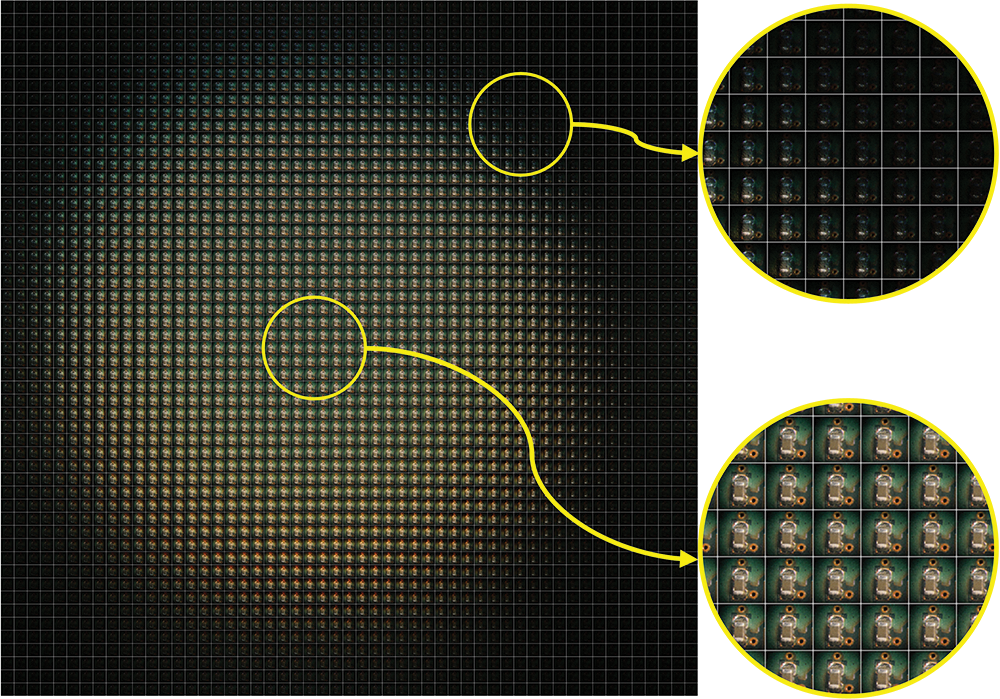
Figure 1: A light field microscopic image with a noise effect

However, it is challenging to reconstruct the complete 3D model of the hidden part from the 2D image. The conventional methods often have difficulty resolving occlusions, which occur when some parts of the scene are obscured and cannot be accurately reconstructed. A reconstructed point cloud can be affected by noise in the input data, leading to errors. Furthermore, some parts of the LF images have low texture and reflective surface information, which can reduce the visual appeal of the reconstructed model. This can make it challenging to accurately align the different views and reconstruct the 3D geometry as shown in Fig. 1. Regarding the solution to such 3D reconstruction problems, DL networks can use many data-driven methods to solve 3D reconstruction problems, especially depth map-based point cloud representation. Therefore, LF imaging systems are used in many computer vision studies since only a small amount of post-processing can provide 3D depth and shape information.

The research presents several critical innovations in the field of 3D reconstruction, including developing a technique for obtaining a 3D point cloud derived from an LF image captured by an LFM camera. Overall, it is a unique method for improving the accuracy of depth maps using a fully convolutional neural network, effectively eliminating noise. In addition, a conversion process that transforms enhanced depth maps into 3D point clouds contributes highly valuable to remote sensing research.

2  Background of LFM and Related Work

2.1 Light Field Microscopy

A conventional optical microscope captures all rays by a single camera sensor from a specific point of view on the sample without directional information. However, when an MLA is inserted into the image plane of an LFM system, it captures a wide range of disparities. Primarily, the LFM system includes a conventional microscope, an MLA, and an image sensor plane. Fig. 2 depicts a schematic diagram of a comprehensive LFM system.

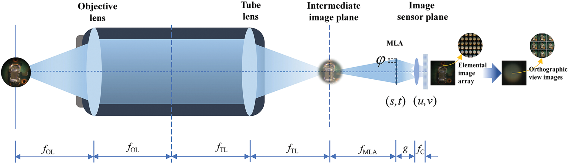
Figure 2: A graphical representation of the LFM system and image-capturing mechanism that utilizes microlens arrays positioned in front of the camera sensor to capture EIA

A light beam is reflected through the objective and tube lenses from a specimen in the intermediate image plane. From this plane, EIA is constructed in front of the camera lens (CL). Geometric analysis is required to calculate the disparity between two elemental images (EI) using parallax information that varies slightly between the images. The OVI is computed using EIA from disparity data. Based on Eq. (1), the point (x, y, z) of an object is mapped to the EIA plane by the CL and the elemental lens (EL).

XEI(i,j)=fMLAfC(i×φ−x)−fCi×φ(z−fMLA)(g−fMLA)(z−fMLA)YEI(i,j)=fMLAfC(j×φ−y)−fCj×φ(z−fMLA)(g−fMLA)(z−fMLA)(1)

Here, fC, and fMLA are the focal length of the camera lens, and the microlens array, respectively. In this case, φ is the length of EL. The focal lengths for an objective and tube lens are fOL and fTL, respectively. A distance of g separates the camera lens from the MLA. i and j indicate the positions of the lenses. Eq. (2) determines the disparity between the EL and CL.

ΔXI=fMLAfCφ(i2−i1)(g−fMLA)(z−fMLA)ΔYI=fMLAfCφ(j2−j1)(g−fMLA)(z−fMLA)(2)

2.2 Related Work

The point cloud stores the geometry of any 3D shape of any object, which is essential to 3D data structures. There are several methods for obtaining a 3D point cloud. Currently, the 3D reconstruction algorithm is divided into voxel [18,19], grid [20], and point cloud-based [21–23] approaches. There are some limitations to the first two methods. For example, opacity and blurring of 3D geometric calculations affect voxel expression. Grid-based reconstruction leads to uneven curve connections, incorrect reconstruction of shapes, and sparse reconstruction. In contrast, a point cloud-based 3D reconstruction is more efficient than the two methods mentioned above. Since point cloud models have a simple data structure that is easily adaptable to training networks. Therefore, DL-based models are considered for point cloud 3D models. To solve the above problems, Lin et al. [24] performed 2D convolution operations to identify the most efficient and optimal network for the 3D reconstruction of single images. A pseudo-rendered depth image was utilized for 2D projection optimization to learn dense 3D shapes. In Yang et al. [25] analysis, the point cloud model was observed with the help of distribution in two stages. The initial stage entails shaping, whereas the subsequent stage pertains to the distribution of points. PointNet [26] and PointNet++ [27] are designed to learn effective representations using equivariant set aggregation and pointwise multi-layer perceptions (MLPs). However, this method does not adequately capture relations between points. PointConv [28] uses a discrete convolutional-based architecture of deep CNN for addressing irregular and unordered point clouds. According to this method, convolutional kernels are constructed on regular grids, with weights related to offsets from the center point. DGCNN [29] designs an EdgeConv capable of extracting features from local shapes of point clouds while maintaining invariance. Although this method is efficient regarding synthetic data, it fails to work on real-world objects.

Gao et al. [30] presented for accurately estimating depth in (LF) images by calculating the slope of EPIs through a directional relationship model and attention mechanism. The proposed algorithm’s effectiveness is demonstrated through outperforming existing algorithms and its potential for use in various LF-related applications, including 3D reconstruction, target detection, and tracking. Luo et al. [31] suggested a CNN model to ascertain the disparity of every pixel, followed by obtaining a group of EPI patches in an LF. Subpixel displacements and occlusions are the main objectives of this method. Using a global constraint, the output of CNN is refined after post-processing. Shin et al. [32] designed a multi-stream neural network that yields epipolar properties from four viewpoints. The convolutional blocks comprise three blocks, each containing a ‘Conv-ReLU-Conv-BN-ReLU’ layer for each branch. The subsequent algorithm branch implements eight more blocks of the same unit layer. Finally, the network ends with a stage encompassing a ‘Conv-ReLU-Conv’ block.

3  Proposed Method for LFM Depth Estimation

The complete procedure comprises three stages: first, image-capturing using the LFM system, as displayed in Fig. 2; second, depth estimation utilizing a deep learning network, and finally, generation of a 3D point cloud from a depth map, as depicted in Fig. 3. EIA is created with MLA by providing a perspective view image. Since the EIA cannot be applied directly to a DL model, it must be generalized as a dataset format. An OVI is then constructed based on the information yielded from the EIA, including data concerning the directional view.

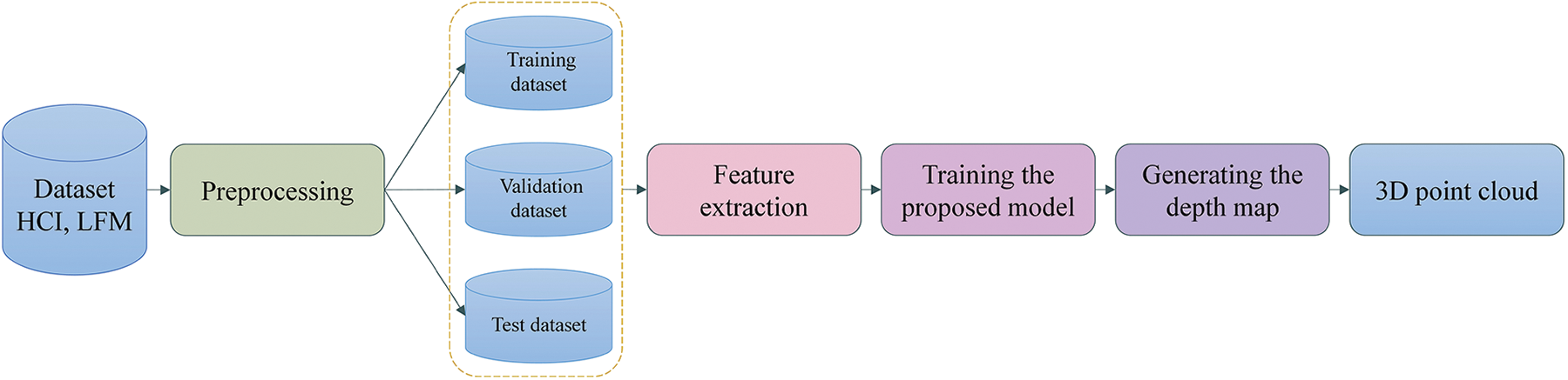
Figure 3: A schematic and workflow diagram of the overall process of 3D reconstruction using a deep learning method

3.1 Dataset Acquisition

Training the network in the proposed model is done with a representative dataset. A synthesized LF data frame is employed in the designed network to achieve the desired result. LF images are significantly larger than traditional stereo images because of their higher angular resolution. The local disparities were estimated with several conventional methodologies, including horizontal, vertical, and diagonal viewpoint EPIs.

This experiment enacts images containing four distinct perspectives (horizontal, vertical, and diagonal) to produce multi-orientation EPIs. A parametric network that can be adjusted according to spatial dimensions is proposed for EPI cuboids with a measurement of 9 × height (h) × width (w) × 3 as input. It has been converted into a smaller size since EPI is 512 by 512. Data cuboids are used for training, testing, and validating EPIs to speed up the training process. The height and width of each cuboid are 32. While crafting the binary dataset, the stride of 13 is used to iterate through the initial image data. As a result, each scene had a total of 38 × 38 = 1444 EPI cuboids. Each EPI cuboid is stored as a piece of data in a binary file, as shown in Fig. 4. Then, each scene is trained and tested using 1444 binary files.

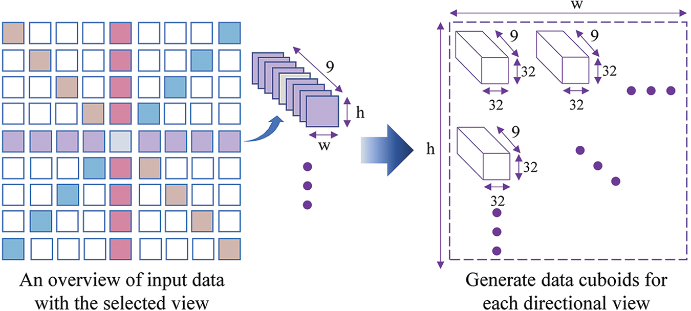
Figure 4: The process of acquiring data for the proposed deep neural network

3.2 Network Architecture

Fig. 5 illustrates the proposed CNN structure. The network consists of four branches as inputs to the four branches, horizontal, vertical, and diagonal data cuboids are used. During the preprocessing, two steps are involved. Initially, zero-mean normalization is applied in each batch to the training dataset, indicating the differences in EPI lines and making the learning process faster for the network. 3D convolution with four-by-four padding is applied next to preserve the attribute map’s spatial dimension. Each branch of the network includes four 3D convolution blocks with activation function ReLU, padding VALID, and stride size 1. The initial two convolution blocks, followed by the third and the fourth, generate 32, 32, 64, and 128 feature maps, respectively. A squeezing layer is then applied. Following the concatenation of the four branches, a convolutional neural network is constructed to become the next layer. After concatenating 3D-CNN, the U-net architecture adds five convolutional blocks to process the data. The first two blocks of the U-net consist of ‘C-B-C-B-C’ operations. A max-pooling layer follows each of these two blocks. Provided that early simulation outcomes indicated a decrease in convergence speed with additional layers, two convolutional (‘C-C’) layers are appended without activation function in the three subsequent blocks of the U-net. An up-sampling layer follows each of these blocks. The first and last convolution blocks generate 64 feature maps, 128 feature maps generated by the second and fourth blocks, and 256 feature maps generated by the third block. A ReLU activation is performed on each convolutional block in the U-net. The final step is to add five more 2D convolutional layers at the tail end of the architecture, which lead to 32, 32, 16, 8, and 1 feature maps and a squeezing layer, respectively, with the kernel 3 × 3 and the padding SAME.

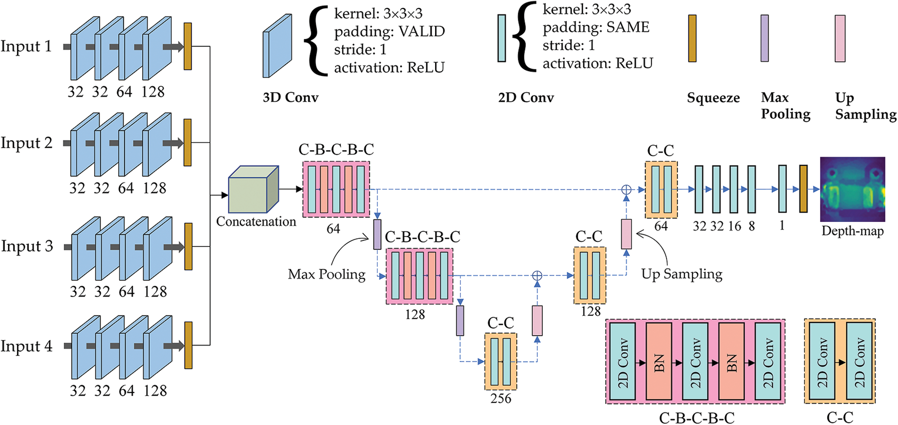
Figure 5: An enhanced depth estimation network architecture

The parameters are trained for 1000 epochs with a learning rate of 1 × 10−4, and the learning decay rate is adjusted by a factor of 0.8 every 50 epochs. Each epoch takes approximately 80–90 s to complete. The total parameters and average runtime of the proposed model are 3,623,777 and 2.49 s for the LFM dataset, respectively. After training, the output is processed using a dual iteration-based weighted median filtering (WMF) method to remove internal noise while preserving pixel information about the edge of the image. The WMF filter is a median filter, which replaces a pixel’s value with the median value of its neighbors. This results in a higher-quality depth estimation image, as shown in Fig. 6.

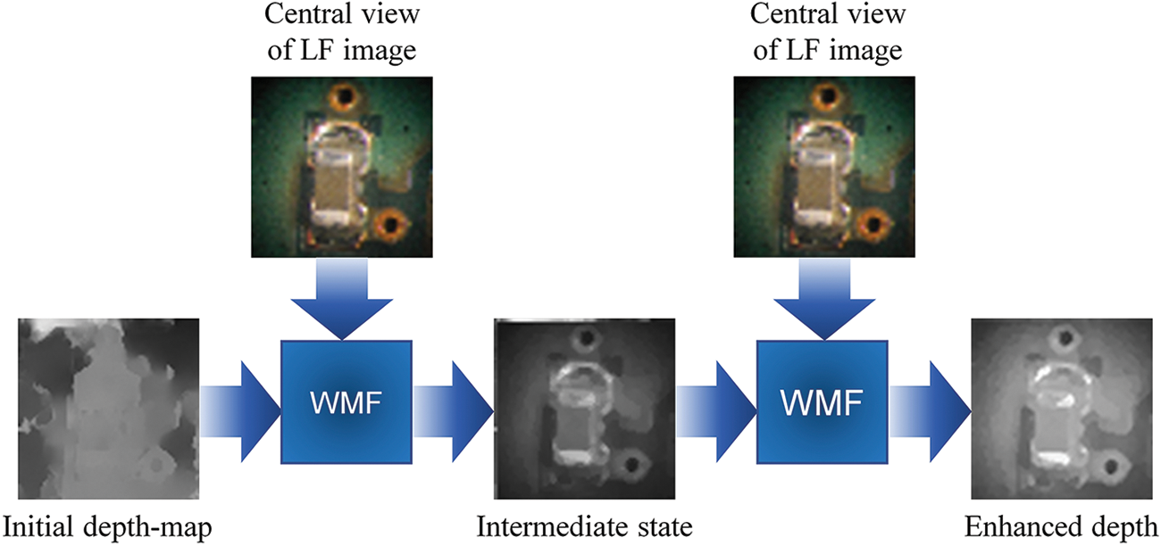
Figure 6: The filter (WMF) reduces internal noise

3.3 3D Reconstruction Using Depth Map

The point cloud model is calculated by transforming the depth pixels from the depth image in the 2D coordinate system to the 3D coordinate system (x, y, z). The model can be constructed by interpolating a depth map, where the z factor of each point at (u, v) represents the point cloud data. The 2D color image and the corresponding estimated depth image are stored in a matrix arrangement. The final point cloud is computed using the following Eq. (3), where (u, v) denotes the depth value at the row u and column v.

x=(u−cx)×zfx,y=(v−cy)×zfy,z=depth(u,v),(3)

Here, the focal lengths are fx, fy, and the optical centers are cx, cy. Point clouds (Pxyz) can be described as follows:

Pxyz=Pi(xi,yi,zi)(4)

where x, y, and z are the 3D coordinates, and i is the number of points.

3.4 Loss Function

Ground truth values are extremely accurate for performance evaluation and disparity measurement in 4D light-field HCI benchmarks [33]. Mean absolute error is a robust loss function not affected by outliers, making it suitable for tasks involving potentially extreme prediction errors. The mean absolute error (MAE) [34] loss function is a commonly used regression loss function that measures the average absolute difference between the predicted values (p^i) and the ground truth value (gi). It is defined as follows:

LossMAE=1N∑i=1N⁡|p^i−gi|(5)

Here, N is the number of errors, and i is the number of examinations.

4  Experiment and Discussion

The following section provides an overview of the datasets used for training and evaluation. The evaluation matrix was then described in detail. The results are presented in both quantitative and qualitative formats. Finally, the results are compared with state-of-the-art techniques.

4.1 Evaluation Metric

There are different methods available to assess the quality of a generated image by comparing it to the original image.

4.1.1 Discrete Entropy

Discrete entropy (DE) [35] measures the uncertainty or randomness in a discrete random variable. The randomness of the variable quantifies the amount of information generated by a random variable. Therefore, better performance is represented by a higher score. A DE index is used as the quantitative measure of the contrast improvement, which is calculated as follows:

DE=−∑i=1n⁡p(xi)×log2⁡p(xi)(6)

Here, the number of grayscales is identified by i, while the probability of each grayscale is represented by p(xi).

4.1.2 Structural Similarity Index

The SSIM [36] is a method for measuring the structural similarity of two images. It is based on the mean, standard deviation, and cross-covariance of the two images, and it is robust to changes in lighting and contrast, making it a good measure of perceived image quality.

SSIM(x,y)=(2∗μx∗μy+C1)∗(2∗σxy+C2)(μx2+μy2+C1)∗(σx2+σy2+C2)(7)

where x and y are the two images being compared, μx and μy are the means of the two images, σx2 and σy2 are the variances of the two images, σxy is the covariance of the two images, C1 and C2 are constants used to avoid instability.

4.1.3 Point Density

In a 3D reconstruction, point density [37] refers to the number of 3D points per unit area or volume. The measurement is commonly expressed as points per unit volume (cubic unit). Points are more evenly distributed when the point density is lower.

Point density=∑in⁡PiVt(8)

In this case, Pi refers to the total number of points on the object’s surface, while Vt refers to the total volume of the region.

4.2 Datasets

Comparative evaluations of methods to estimate disparity for light field images are often conducted using the HCI benchmark [33]. Since no datasets exist for the LFM system, the proposed network was trained on the HCI dataset comprising 24 scenes. The training set consisted of 15 scenes, with four scenes used for validation and the remaining scenes reserved for testing. Blender is used to render the benchmark LF images. There are a variety of materials, lighting conditions, and delicate structures with complex occlusions in the scenes included in this dataset. Images are of resolution 512 × 512, with nine sub-aperture views in each direction. All scenes contain 8 bits of light field data, camera parameters, and depth information. This benchmark is specifically designed to address challenges that present difficulties in 3D models, such as depth estimation, occlusions of boundaries, geometry structures, lack of smooth surfaces, background noise, and low-texture images.

A depth evaluation-based 3D reconstruction model is proposed utilizing the LFM data. The LFM scene contains 53 by 53 directional-view images, with each view composed of 75 by 75 pixels. A region of interest (ROI) is taken for each OVI, and 9 × 9 angular images are used to calculate the depth field of each OVI. The generation of test data involves taking nine images at intervals of three images in each direction, as shown in Fig. 7.

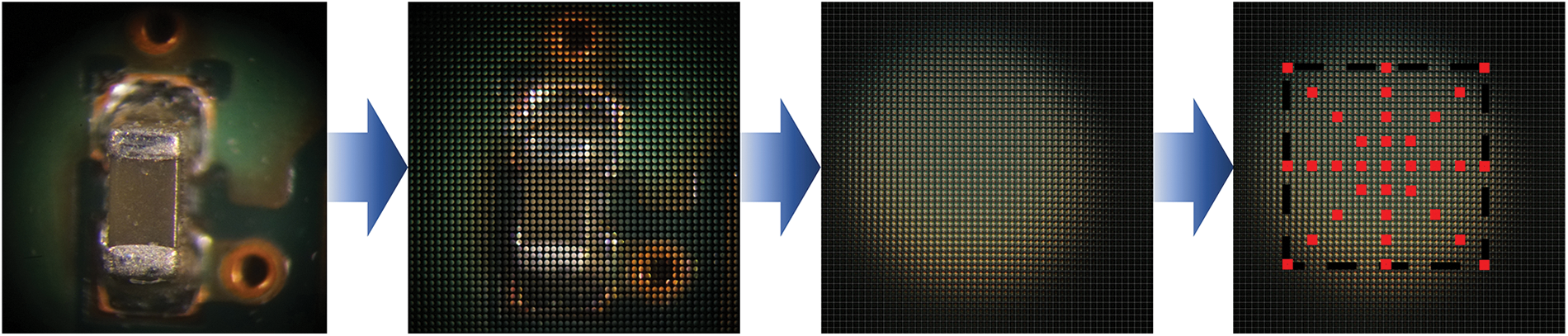
Figure 7: Generating test data from LF the microscopic specimen

4.3 Implementation Details

This study uses an optical system with infinity correction (Olympus SZX7 microscope, Olympus Corporation, Tokyo, Japan) with a 1× magnification. It employs an array of 100 × 100 MLA with a diameter of 2.4 mm and a focal length of 125 μm for LFM. An image is captured with a Sony α6000 camera with a sensor resolution of 6000 × 4000 pixels. LFM data can be captured at 4028 × 4028 pixels. The optical setup is shown in Fig. 8.

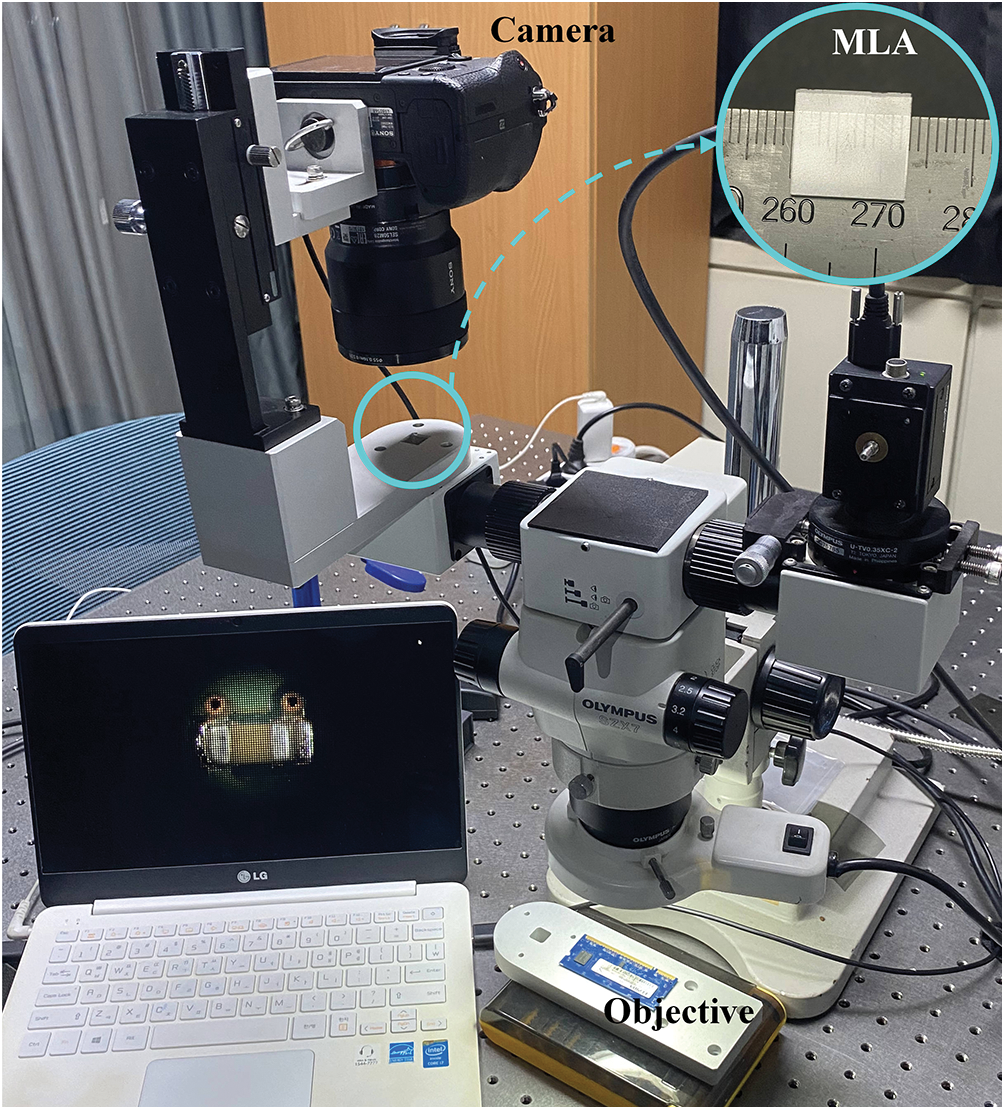
Figure 8: An optical system for capturing light field microscopic images

The proposed model is being trained on a Windows 10 Pro 64-bit machine equipped with an Intel Core i7-9800X 3.80 GHz processor, 128 GB of memory, and an NVIDIA GeForce RTX 2080 Ti GPU. During the training and testing of this network, Python is used with the TensorFlow library. As shown in Fig. 9, the training loss and validation graphs are plotted. The proposed model is being tested using different size real-world LFM images.

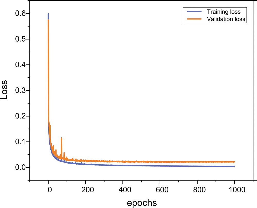
Figure 9: Training and validation loss of the proposed training model

4.4 Results Analysis

Different types of synthetic and real objects were used in this experiment. Using the HCI dataset, disparity maps are estimated for synthetic data experiments. SSIM and mean squared errors (MSE) values are used as a way of evaluating our method. An evaluation of SSIM values was performed compared with five state-of-the-art methods. In these cases, our method is compared with OACC-Net [38], LLF-Net [39], MA-Net [40], LFatt-Net [41], and EPI-Net [32]. The quantitative evaluation results are shown in Table 1. This table shows that our approach has an average result of approximately 2%, 4%, and 5% better than OACC-Net, MA-Net, and LFatt-Net, respectively. However, it is noteworthy that it is around 42% better than EPI-Net and LLF-Net, indicating a significant improvement. As test images, boxes, cotton, pillows, and pens images data are considered. A visual comparison between the five methods and the proposed methods is shown in Fig. 10.

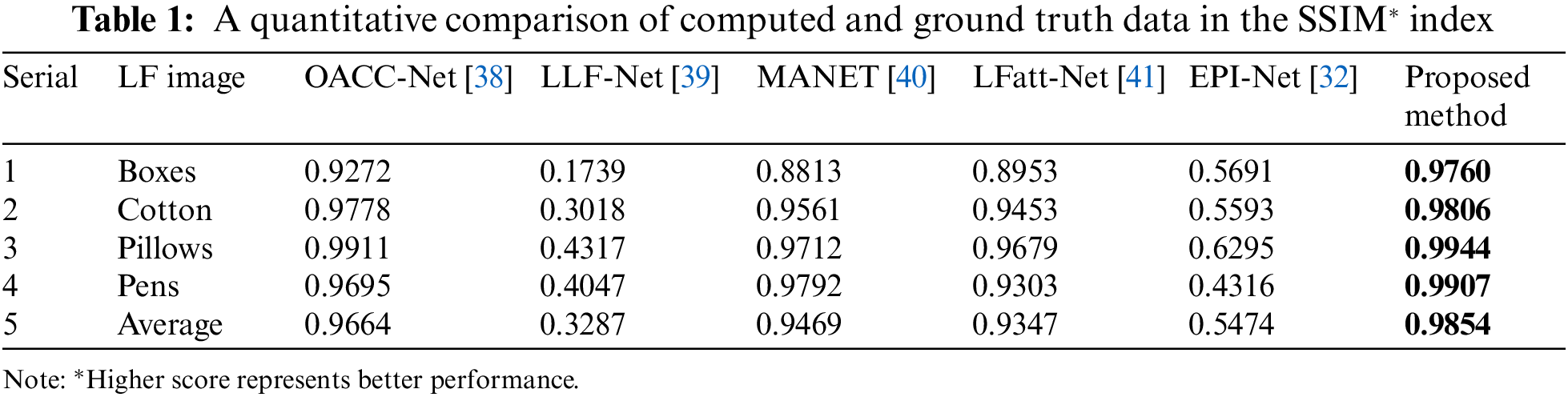
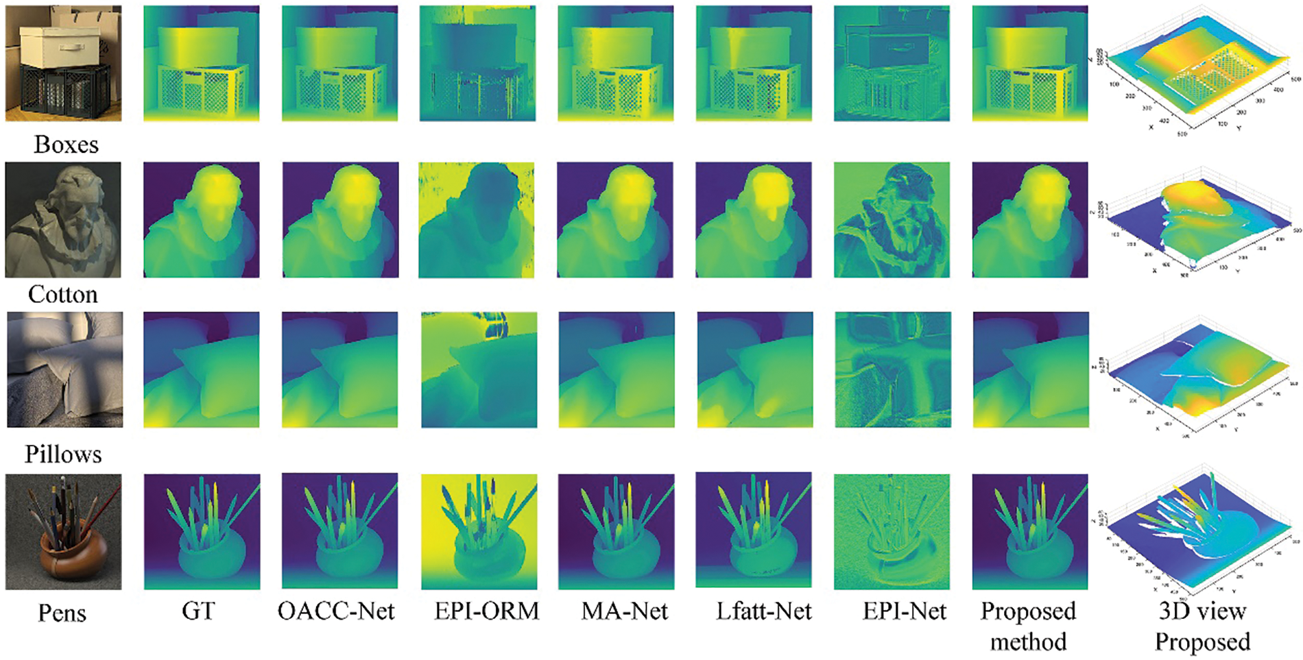
Figure 10: Visual results for LF depth images of four objects with ground truth disparity. (1st column) RGB images and (2nd column) ground truth (GT) disparity. (3rd column) OACC-Net results. (4th column) LLF-Net results. (5th column) MA-Net results. (6th column) LFatt-Net results. (7th column) EPI-Net results. (8th column) Proposed method results. (9th column) Proposed method results of the 3D point cloud

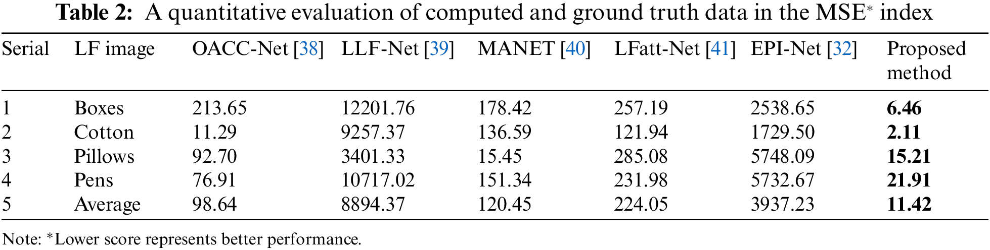
Table 2 presents the MSE values for depth images of the HCI data. For the Boxes, Cotton, Pillows, and Pens, the MSE values of depth map images by the proposed method are 6.46, 2.11, 15.21, and 21.91, respectively.

We compare our LF depth estimation results with five existing algorithms for evaluation. In these cases, OACC-Net, LLF-Net, MA-Net, LFatt-Net, and EPI-Net methods are assessed with a DE test. Fig. 11 (1st column) illustrates the specimens. The DE index is used for enhanced depth quality since real objects do not have ground truth values. Compared to existing methods, the DE formula showed better contrast in the depth map. The DE values for the (a) integrated circuit (IC)-1, (b) IC-2, (c) Chip [42], and (d) Micro Gear [43], are 8.38, 8.11, 8.84, and 8.19, respectively. In this case, the entropy values of (4.99, 1.38, 6.23, and 4.84) are for the OACC-Net, (3.86, 3.36, 2.65, and 7.64) for the LLF-Net, (3.86, 4.95, 4.27, and 7.97) for the MA-Net, (6.68, 6.68, 6.83, and 6.43) for the LFatt-Net, and (7.07, 6.94, 7.19, and 7.12) for EPI-Net method, respectively as shown in Fig. 12. Compared to existing methods, the proposed model-driven depth map calculation method produces a 3D representation that is clearer and more accurate.

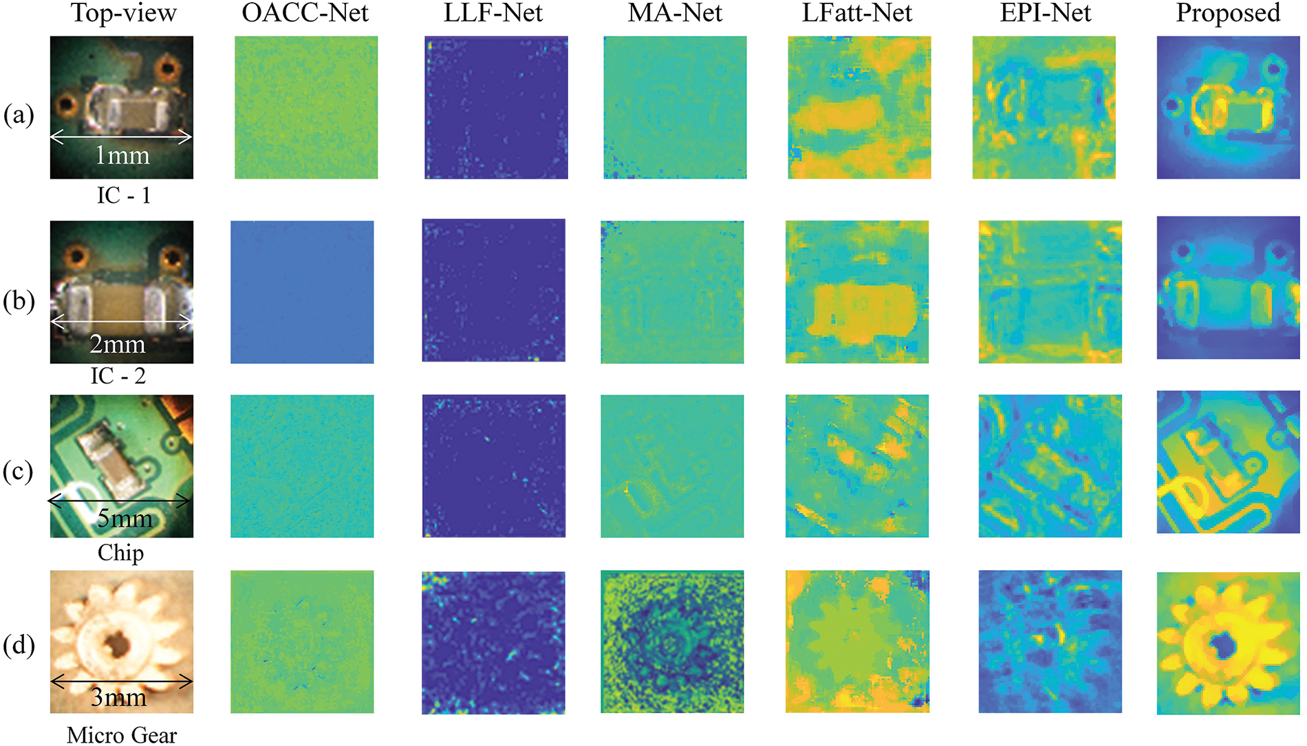
Figure 11: Visual results for the central view of four LFM depth images, from top to bottom: (a) integrated circuit (IC)-1 (1 mm), (b) IC-2 (2 mm), (c) chip (5 mm), and (d) micro gear (3 mm)

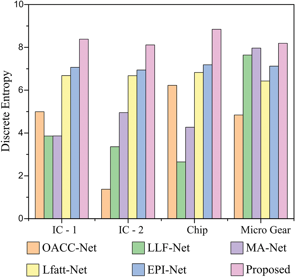
Figure 12: Quantitative comparison of LFM depth map computation using discrete entropy index

The reconstructed 3D point cloud models are depicted in Fig. 13, based on the predicted depth map and point cloud interpolation. Table 3 presents the point cloud density values for 3D reconstructed images. For the IC-1, IC-2, Chip, and Micro Gear, the point cloud density values of reconstructed 3D images by the proposed method are 0.0066, 0.0005, 0.0002, and 0.0021, respectively. The results demonstrate the accuracy of the suggested technique in replicating the depth images. As a result, the proposed U-Net-based CNN outperformed previous deep-learning methods for the LFM system.

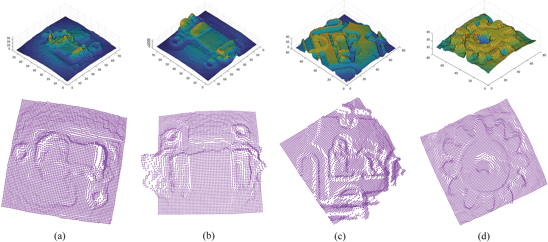
Figure 13: Proposed three-dimensional depth map and reconstructed point cloud 3D images

The proposed application of the DL technique for enhancing the reconstruction of 3D point clouds in LFM is promising. However, it has certain limitations. The proposed approach depends on high-quality directional data. Despite this model showing excellent performance, its trainable parameters are high, which makes training the network more challenging. Additionally, when converting the EIA to OVI, the size of directional images reduces. Furthermore, the proposed method’s computational cost and number of training parameters are high, particularly when handling large datasets.

5  Conclusion

The paper introduces a new approach for 3D point cloud reconstruction using LFM image data that leverages the DL technique. The proposed method employs a fully convolutional neural network to extract and utilize geometry structure and edge information from the LFM images. A 3D point cloud reconstruction method based on DL can overcome the limitations of traditional methods, such as low resolution, noise sensitivity, and occlusions. The data for this method is collected using a camera sensor and a lens array in combination with a 2D optical microscope and then processed to generate an OVI using a pixel mapping algorithm. The directional LF image is collected from the ROI to overcome the inconsistency of brightness. The proposed network extracts the depth map using the collected LFM data and U-Net-based CNN. After that, the proposed method uses a dual iteration-based weighted median filtering approach for depth map enhancement. Finally, a 3D reconstructed point cloud is generated by interpolating a depth map. This technique performs better than existing algorithms. Furthermore, the article compares the effectiveness of the proposed algorithm with well-established DL algorithms for evaluation purposes. Despite this, further research is required to address issues such as insufficient annotated training and test dataset. Our future work in this area will focus on developing robust methods for solving existing drawbacks and datasets using deep-learning techniques.

Acknowledgement: The authors would like to thank all our colleagues who assisted us in completing the manuscript and provided technical and mental support throughout the process.

Funding Statement: This research was supported by the National Research Foundation of Korea (NRF) (NRF-2018R1D1A3B07044041 & NRF-2020R1A2C1101258), and supported by the MSIT (Ministry of Science and ICT), Korea, under the ITRC (Information Technology Research Center) Support Program (IITP-2023-2020-0-01846), was conducted during the research year of Chungbuk National University in 2023.

Author Contributions: The authors confirm their contribution to the paper as follows: Study conception and design: S.M. Imtiaz; data collection: S.M. Imtiaz, M.B. Hossain, R.K. Shinde; analysis and interpretation of results: S.M. Imtiaz; K.C. Kwon, N. Kim; draft manuscript preparation: S.M. Imtiaz, F.M.F. Hossain, K.C. Kwon, S.K. Gil, N. Kim. All authors reviewed the results and approved the final version of the manuscript.

Availability of Data and Materials: The datasets utilized in this paper are publicly available. Additionally, we offer the evaluation codes and test codes for the proposed method, which can be accessed at: https://github.com/shariarmdimtiaz/LFM-3D-Point-Cloud-Reconstruction (Accessed on 25 April 2023).

Conflicts of Interest: The authors declare that they have no conflicts of interest to report regarding the present study.

References

1. M. Levoy, R. Ng, A. Adams, M. Footer and M. Horowitz, “Light field microscopy,” in Special Interest Group on Computer Graphics and Interactive Techniques Conf. (SIGGRAPH), New York, NY, USA, pp. 924–934, 2006. https://doi.org/10.1145/1179352.1141976 [Google Scholar] [CrossRef]

2. M. Levoy and P. Hanrahan, “Light field rendering,” in Proc. of the 23rd Annual Conf. on Computer Graphics and Interactive Techniques, New Orleans, Louisiana, USA, pp. 31–42, 1996. [Google Scholar]

3. M. Martínez-Corral and B. Javidi, “Fundamentals of 3D imaging and displays: A tutorial on integral imaging, light-field, and plenoptic systems,” Advances in Optics and Photonics, vol. 10, no. 3, pp. 512, 2018. https://doi.org/10.1364/AOP.10.000512 [Google Scholar] [CrossRef]

4. Y. Du, Q. Zhang, D. Hua, J. Hou, B. Wang et al., “EANet: Depth estimation based on epi of light field,” Biomed Research International, vol. 2021, pp. 1–10, 2021. https://doi.org/10.1155/2021/8293151 [Google Scholar] [PubMed] [CrossRef]

5. K. C. Kwon, J. S. Jeong, M. U. Erdenebat, Y. T. Lim, K. H. Yoo et al., “Real-time interactive display for integral imaging microscopy,” Applied Optics, vol. 53, no. 20, pp. 4450, 2014. https://doi.org/10.1364/AO.53.004450 [Google Scholar] [PubMed] [CrossRef]

6. C. Zheng, X. Yan, H. Zhang, B. Wang, S. Cheng et al., “Beyond 3D siamese tracking: A motion-centric paradigm for 3D single object tracking in point clouds,” in Proc. of the IEEE/CVF Conf. on Computer Vision and Pattern Recognition, New Orleans, Louisiana, USA, pp. 8111–8120, 2022. https://doi.org/10.48550/arXiv.2203.01730 [Google Scholar] [CrossRef]

7. C. R. Qi, H. Su, K. Mo and L. J. Guibas, “PointNet: Deep learning on point sets for 3D classification and segmentation,” in Proc. of the IEEE Conf. on Computer Vision and Pattern Recognition, Honolulu, HI, USA, pp. 652–660, 2017. https://doi.org/10.48550/arXiv.1612.00593 [Google Scholar] [CrossRef]

8. Y. Wei, Z. Ding, H. Huang, C. Yan, J. Huang et al., “A Non-contact measurement method of ship block using image-based 3D reconstruction technology,” Ocean Engineering, vol. 178, pp. 463–475, 2019. https://doi.org/10.1016/j.oceaneng.2019.03.015 [Google Scholar] [CrossRef]

9. T. Zhang and Y. Cao, “Improved lightweight deep learning algorithm in 3D reconstruction,” Computers, Materials & Continua, vol. 72, no. 3, pp. 5315–5325, 2022. https://doi.org/10.32604/cmc.2022.027083 [Google Scholar] [CrossRef]

10. D. D. Gregorio and L. D. Stefano, “SkiMap: An efficient mapping framework for robot navigation,” in Proc. IEEE Int. Conf. on Robotics and Automation (ICRA), Marina Bay Sands, Singapore, pp. 2569–2576, 2017. https://doi.org/10.1109/ICRA.2017.7989299 [Google Scholar] [CrossRef]

11. S. M. Imtiaz, K. C. Kwon, M. Alam, M. Hossain, N. Changsup et al., “Identification and correction of microlens-array error in an integral-imaging-microscopy system,” Current Optics and Photonics, vol. 5, no. 5, pp. 524–531, 2021. https://doi.org/10.3807/COPP.2021.5.5.524 [Google Scholar] [CrossRef]

12. A. Nwaneshiudu, C. Kuschal, F. H. Sakamoto, R. R. Anderson, K. Schwarzenberger et al., “Introduction to confocal microscopy,” Journal of Investigative Dermatology, vol. 132, no. 12, pp. 1–5, 2012. https://doi.org/10.1038/jid.2012.429 [Google Scholar] [PubMed] [CrossRef]

13. A. D. Elliott, “Confocal microscopy: Principles and modern practices,” Current Protocols in Cytometry, vol. 92, no. 1, pp. e68, 2020. https://doi.org/10.1002/cpcy.68 [Google Scholar] [PubMed] [CrossRef]

14. Y. Long, J. Zhang, Z. Liu, W. Feng, S. Guo et al., “Metalens-based stereoscopic microscope,” Photonics Research, vol. 10, no. 6, pp. 1501–1508, 2022. https://doi.org/10.1364/PRJ.456638 [Google Scholar] [CrossRef]

15. S. Barkley, T. G. Dimiduk, J. Fung, D. M. Kaz, V. N. Manoharan et al., “Holographic microscopy with python and holopy,” Computing in Science & Engineering, vol. 22, no. 5, pp. 72–82, 2020. https://doi.org/10.1109/MCSE.2019.2923974 [Google Scholar] [CrossRef]

16. K. C. Kwon, K. H. Kwon, M. U. Erdenebat, Y. L. Piao, Y. T. Lim et al., “Advanced three-dimensional visualization system for an integral imaging microscope using a fully convolutional depth estimation network,” IEEE Photonics Journal, vol. 12, no. 4, pp. 1–14, 2020. https://doi.org/10.1109/JPHOT.2020.3010319 [Google Scholar] [CrossRef]

17. H. Farhood, S. Perry, E. Cheng and J. Kim, “Enhanced 3D point cloud from a light field image,” Remote Sensing, vol. 12, no. 7, pp. 1125, 2020. https://doi.org/10.3390/rs12071125 [Google Scholar] [CrossRef]

18. R. Tahir, A. B. Sargano and Z. Habib, “Voxel-based 3D object reconstruction from single 2D image using variational autoencoders,” Mathematics, vol. 9, no. 18, pp. 2288, 2021. https://doi.org/10.3390/math9182288 [Google Scholar] [CrossRef]

19. K. Peng, R. Islam, J. Quarles and K. Desai, “TMVNet: Using transformers for multi-view voxel-based 3D reconstruction,” in Proc. of the IEEE/CVF Conf. on Computer Vision and Pattern Recognition, New Orleans, Louisiana, USA, pp. 222–230, 2022. [Google Scholar]

20. V. A. Knyaz, V. V. Kniaz, F. Remondino, S. Y. Zheltov and A. Gruen, “3D reconstruction of a complex grid structure combining uas images and deep learning,” Remote Sensing, vol. 12, no. 19, pp. 3128, 2020. https://doi.org/10.3390/rs12193128 [Google Scholar] [CrossRef]

21. H. Chen, Y. Zuo, Y. Tong and L. Zhu, “3D point cloud generation reconstruction from single image based on image retrieval,” Results in Optics, vol. 5, pp. 100124, 2021. https://doi.org/10.1016/j.rio.2021.100124 [Google Scholar] [CrossRef]

22. S. M. Imtiaz, K. C. Kwon, M. B. Hossain, M. S. Alam, S. H. Jeon et al., “Depth estimation for integral imaging microscopy using a 3D–2D CNN with a weighted median filter,” Sensors, vol. 22, no. 14, pp. 5288, 2022. https://doi.org/10.3390/s22145288 [Google Scholar] [PubMed] [CrossRef]

23. J. Zhang, X. Qi, S. H. Myint and Z. Wen, “Deep-learning-empowered 3D reconstruction for dehazed images in IoT-enhanced smart cities,” Computers, Materials & Continua, vol. 68, no. 2, pp. 2807–2824, 2021. https://doi.org/10.32604/cmc.2021.017410 [Google Scholar] [CrossRef]

24. C. H. Lin, C. Kong and S. Lucey, “Learning efficient point cloud generation for dense 3D object reconstruction,” in Proc. of the AAAI Conf. on Artificial Intelligence, Louisiana, USA, vol. 32, no. 1, pp. 7114–7121, 2018. [Google Scholar]

25. G. Yang, X. Huang, Z. Hao, M. Y. Liu, S. Belongie et al., “PointFlow: 3D point cloud generation with continuous normalizing flows,” in Proc. of the IEEE/CVF Int. Conf. on Computer Vision, Seoul, Rep. of Korea, pp. 4541–4550, 2019. [Google Scholar]

26. C. R. Qi, H. Su, K. Mo and L. J. Guibas, “PointNet: Deep learning on point sets for 3D classification and segmentation,” in Proc. of the IEEE Conf. on Computer Vision and Pattern Recognition (CVPR), Honolulu, HI, USA, pp. 652–660, 2017. [Google Scholar]

27. C. R. Qi, L. Yi, H. Su and L. J. Guibas, “PointNet++: Deep hierarchical feature learning on point sets in a metric space,” in Proc. of the Int. Conf. on Neural Information Processing System, California, CA, USA, pp. 5099–5108, 2017. [Google Scholar]

28. W. Wu, Z. Qi and L. Fuxin, “PointConv: Deep convolutional networks on 3D point clouds,” in Proc. of the IEEE/CVF Conf. on Computer Vision and Pattern Recognition, Seoul, Korea, pp. 9621–9630, 2019. [Google Scholar]

29. Y. Wang, Y. Sun, Z. Liu, S. E. Sarma, M. M. Bronstein et al., “Dynamic graph CNN for learning on point clouds,” Association for Computing Machinery (ACM) Transactions on Graphics, vol. 38, no. 5, pp. 1–12, 2019. [Google Scholar]

30. M. Gao, H. Deng, S. Xiang, J. Wu and Z. He, “EPI light field depth estimation based on a directional relationship model and multiviewpoint attention mechanism,” Sensors, vol. 22, no. 16, pp. 6291, 2022. https://doi.org/10.3390/s22166291 [Google Scholar] [PubMed] [CrossRef]

31. Y. Luo, W. Zhou, J. Fang, L. Liang, H. Zhang et al., “EPI-patch based convolutional neural network for depth estimation on 4D light field,” in Neural Information Processing: 24th Int. Conf. (ICONIP), Guangzhou, China, pp. 642–652, 2017. https://doi.org/10.1007/978-3-319-70090-8_65 [Google Scholar] [CrossRef]

32. C. Shin, H. G. Jeon, Y. Yoon, I. S. Kweon and S. J. Kim, “EPINET: A fully-convolutional neural network using epipolar geometry for depth from light field images,” in Proc. of the IEEE Conf. on Computer Vision and Pattern Recognition, Salt Lake City, UT, USA, pp. 4748–4757, 2018. [Google Scholar]

33. K. Honauer, O. Johannsen, D. Kondermann and B. Goldluecke, “A dataset and evaluation methodology for depth estimation on 4D light fields,” in Proc. of Asian Conf. on Computer Vision (ACCV), Taipei, Taiwan, pp. 19–34, 2016. https://doi.org/10.1007/978-3-319-54187-7_2 [Google Scholar] [CrossRef]

34. T. Chai and R. R. Draxler, “Root mean square error (RMSE) or mean absolute error (MAE),” Geoscientific Model Development Discussions, vol. 7, no. 3, pp. 1247–1250, 2014. [Google Scholar]

35. B. H. Kim, C. Bohak, K. H. Kwon and M. Y. Kim, “Cross fusion-based low dynamic and saturated image enhancement for infrared search and tracking systems,” IEEE Access, vol. 8, pp. 15347–15359, 2020. https://doi.org/10.1109/ACCESS.2020.2966794 [Google Scholar] [CrossRef]

36. I. Bakurov, M. Buzzelli, R. Schettini, M. Castelli and L. Vanneschi, “Structural similarity index (SSIM) revisited: A data-driven approach,” Expert Systems with Applications, vol. 189, pp. 116087, 2022. [Google Scholar]

37. Z. Liu, D. Kim, S. Lee, L. Zhou, X. An et al., “Near real-time 3D reconstruction and quality 3D point cloud for time-critical construction monitoring,” Buildings, vol. 13, no. 2, pp. 464, 2023. https://doi.org/10.3390/buildings13020464 [Google Scholar] [CrossRef]

38. Y. Wang, L. Wang, Z. Liang, J. Yang, W. An et al., “Occlusion-aware cost constructor for light field depth estimation,” in Proc. of the IEEE/CVF Conf. on Computer Vision and Pattern Recognition, New Orleans, Louisiana, USA, pp. 19809–19818, 2022. [Google Scholar]

39. Y. Li, Q. Wang, L. Zhang and G. Lafruit, “A lightweight depth estimation network for wide-baseline light fields,” IEEE Transactions on Image Processing, vol. 30, pp. 2288–2300, 2021. https://doi.org/10.1109/TIP.2021.3051761 [Google Scholar] [PubMed] [CrossRef]

40. Y. Li, L. Zhang, Q. Wang and G. Lafruit, “Manet: Multi-scale aggregated network for light field depth estimation,” in IEEE Int. Conf. on Acoustics, Speech and Signal Processing (ICASSP), Barcelona, Spain, pp. 1998–2002, 2020. https://doi.org/10.1109/ICASSP40776.2020.9053532 [Google Scholar] [CrossRef]

41. Y. J. Tsai, Y. L. Liu, M. Ouhyoung and Y. Y. Chuang, “Attention-based view selection networks for light-field disparity estimation,” in Proceedings of the AAAI Conference on Artificial Intelligence, vol. 34, no. 7, pp. 12095–12103, 2020. https://doi.org/10.1609/aaai.v34i07.6888 [Google Scholar] [CrossRef]

42. M. S. Alam, K. C. Kwon, M. U. Erdenebat, M. Y. Abbass, M. A. Alam et al., “Super-resolution enhancement method based on generative adversarial network for integral imaging microscopy,” Sensors, vol. 21, no. 6, pp. 2164, 2021. https://doi.org/10.3390/s21062164 [Google Scholar] [PubMed] [CrossRef]

43. K. C. Kwon, M. U. Erdenebat, A. Khuderchuluun, K. H. Kwon, M. Y. Kim et al., “High-quality 3D display system for an integral imaging microscope using a simplified direction-inversed computation based on user interaction,” Optics Letters, vol. 46, no. 20, pp. 5079, 2021. https://doi.org/10.1364/OL.436201 [Google Scholar] [PubMed] [CrossRef]