A Consistent Mistake in Remote Sensing Images’ Classification Literature

1  Introduction

Remote sensing is an important imaging technique for humans observing the earth from space. The interpretation of RSI plays a crucial role in applications. In general, interpreting RSI requires a higher level of real-time processing. However, as the number of orbital sensors grows, the big data from RS cannot be processed manually. As a result, machine learning became the foremost technique for interpreting the RSI [1]. Traditional ML-based methods rely excessively on human-engineered feature indicators [2]. In other words, interpreting the RSI is still labor-intensive and domain-specific, even for ML-based algorithms. Fortunately, this quandary has a suitable solution in the form of deep learning (DL) techniques [3]. The leading characteristic of DL is the automatic feature extraction and end-to-end training procedure.

Different roadmaps have been proposed for the RSI tasks. As an essential part, the semantic classification (SC) application gains most of the attention compared to other tasks, e.g., semantic segmentation [4], object detection [5], and recognition [6]. There have been several technical routes for SC tasks. Deep CNN is gradually gaining traction due to its higher accuracy, controllable capacity, and low hardware cost [7]. Unsurprisingly, the winning CNN story is not immediately apparent.

Firstly, the CNN-based methods are only used as fixed feature extractors for RSI-SC [8]. The models are only pre-trained on natural images, and no customized training strategies or fine-tuning procedures are used. Following that, CNN-based methods changed to transfer-learning strategies, and the majority of them have been fine-tuned on RSI datasets. At that time, deep features fused with handcrafted ones were popular. For example, Chaib et al. proposed a method using discriminate correlation analysis (DCA) for deep features [9]. However, these relevant algorithms are commonly very abstruse and not universal across different datasets. The cause is mainly due to two facts, i.e., the insufficiency of optional CNN architectures and knowledge about CNN’s remarkable representation ability. Afterwards, the pure CNN-based technical line becomes dominant. In the course of the accuracy competition, algorithms consisting of multiple models or feature enhancements govern the research fields [10]. In contrast, the time and hardware costs garner little attention. Only until the transformer arises will the academic community suddenly realize that the training optimization strategy is so important for the CNN models [11].

DL techniques are more discriminative mainly because of the multidimensional affine transformations generated by the top-down, hierarchical deep layers. It is well known that the depth of the CNN model corresponds to more multivariable features, while the width indicates multidimensionality. Arguably, the traditional ML technique is less competitive owing to its limited human-engineered features. Hence, all of the aforementioned methods can be effective, mainly because the algorithm’s indicators have increased. The difference is that the algorithmically extracted features are more efficient than the handcrafted ones. Technically speaking, more attention-structured modules in the CNN’s architecture are a good option to boost the model’s performance. Nevertheless, more discriminative features can be achieved through extensive data samples, too. In fact, data augmentation (DA) techniques are the most widely employed strategies to boost the CNN method’s performance nowadays. For example, Khan et al. proposed a method using a pseudo-example generator to improve the model’s performance [12].

Recently, the author proposed an algorithm to improve a CNN model’s performance for RSI-SC, named the FST-EfficientNet [13]. It employs the smallest architecture of EfficientNet version 2 (EfficientNetV2-S) as the base model. The method outperforms all the other previous methods only by employing a routine transfer learning strategy. More importantly, only classic data augmentation (DA) tricks are included without any handcrafted indicators. Motivated by these findings, the author further examines two dozen previous studies that employed different CNN architectures for tasks in RSI-SC. As a comparable baseline, all the same CNN architectures, datasets, and training ratios used in the literature are trained by the FST-CNN algorithm. Surprisingly, only one of the previous studies significantly exceeded the author’s baseline results. In other words, most of the former literature has achieved suboptimal performance unintentionally. The three contributions of this study are summarized as follows:

Firstly, to the best of our knowledge, this is the first time that the issue of systemically existing suboptimal performance in previous studies has been revealed. Results show that there is a maximal OA gap of 8.35% between the FST-CNN and those methods in the literature, which means a 10% margin in performance. The crucial reasons include the inappropriate training strategy and data-distributing shift introduced by DA.

Secondly, the results demonstrate that the FST-CNN algorithm is efficient and model-agnostic. Consistent performance enhancements across different CNN architectures are obvious compared to methods in the literature. DA is only implemented for the input samples. Hence, the algorithm can be employed on any image classification model to potentially boost performance.

Finally, and most importantly, the results show a standardized training strategy is indeed very meaningful to the research of RSI-SC. Most of the performance evaluation in the literature was conducted based on an inaccurate, suboptimal, and unfair result. It has made most of the previous research findings questionable to some extent. There seems to be a big chance to reshape the patterns of deep learning for RSI-SC.

The remainder of this paper is organized as follows: Section 2 gives a brief review of related works. Section 3 describes the proposed method in detail. Section 4 introduces experimental designs and results. Experimental results are discussed in Section 5. Section 6 presents a conclusion and future work.

2  Related Works

Liu et al. proposed a complex approach focusing on modifications of the classical cross-entropy loss function [14]. In detail, three different CNN models are employed to extract the deep features for the formation of hierarchical Wasserstein distance (HWD) metrics, which are packaged into the cross-entropy loss as a hybrid one. Apparently, information disclosure happens when the validation images are involved in the extraction of deep features. Nonetheless, Liu et al. proposed another similar approach by integrating CNN models with Wasserstein distance (WD) losses [15]. Specifically, the validation images are still treated as the inputs of the deep feature extractors.

Cheng et al. proposed a discriminative CNN (DCNN) approach by defining a relatively slim object function [16]. In detail, the Euclidean distances of the deep features are introduced into the cross-entropy losses as regularization. However, the method’s performance is somehow not ideal. As a competitor, Bazi et al. attribute the return of complex handcrafted features to the vanishing gradient problem that exists in the back propagation procedure [17]. As a solution, an auxiliary loss function is introduced to the model’s shallow layers to tackle the vanishing gradient. As we know, the vanishing gradient problem is commonly relevant to a lot of factors, e.g., the learning rate, activation function, and model capacity.

Zhang et al. propose a cascade algorithm that employs two different CNNs as feature extractors, and then the features are fed into a capsule network (CapsNet) [18]. Zhu et al. propose another attention-based deep feature fusion (ADFF) algorithm [19]. It consists of two CNNs, one as a deep feature extractor and the other as a gradient-attention generator. Besides, Minetto et al. proposed the “Hydra” ensemble [20]. It consists of fourteen CNN models. Model combinations and ensembles outperform other routine algorithms in terms of accuracy. However, the cascade CNN models are truly hardware expensive, too.

With the rise of the transformer [21], the attention mechanism offers a cost-controlled technique to enhance the performance of CNN. Guo et al. proposed a saliency-dual attention network (SDANet) [22]. The spatial attention structure is only placed in the model’s second stage, while the channel attention is placed in the third, fourth, and fifth stages, respectively. Similarly, Tong et al. proposed a channel-attention-based network (CADNet) [23]. The “Squeeze and Excitation” (SE) blocks first proposed by Hu et al. [24] are imported into every stage of the model’s architecture. Guo et al. also proposed a global-local attention network (GLANet) [25]. The difference is that it only consists of two attention branches at the end of the fifth stage, i.e., channel and spatial attention. Similarly, Alhichri et al. proposed another spatial attention network (AttnNet) [26]. As a common feature, these four approaches only introduce a controllable parameter increment to the model. However, a significant improvement in performance is not guaranteed for all of them. In conclusion, the former two perform better than the latter ones.

Attention mapping is also included for RSI-SC. Li et al. proposed a method using the fusion of deep features and class activation maps (CAM) to seek a more discriminative feature representation [27]. Tang et al. proposed a method using pairs of rotated images to achieve an attention-consistent network (ACNet) [28]. The multi-scale deep features are also considered attention patterns. Xie et al. proposed a scale-free CNN (SFCNN) method [29]. It replaces the fixed-parameter full-connected layer with a convolutional operation for arbitrary input sizes. Sun et al. proposed a gated bidirectional network (BDNet) [30]. It employs a bi-directionally connected model to hierarchically aggregate multilayer convolutional features. Li et al. proposed a gated recurrent multi-attention network (GRMANet) [31]. It extracts multilevel features at various stages for input to a deep-gated recurrent unit. Chen et al. proposed another global context-spatial attention network (GCSANet) [32]. It consists of multi-scale feature extraction and context modeling. In a word, these five atypical attention methods do achieve ordinary performance, though the algorithm’s procedure seems abstruse.

Recently, training optimization strategies have boomed. Howard proposes a “progressive resizing” method by increasing image size in successive training epochs [33]. This method offers convenient multi-scale features, though its accuracy is not ideal. Hoffer et al. propose a “mix and match” method by using stochastic images and batch sizes through random sampling to improve the algorithm’s robustness and training efficiency [34]. This method applies effects like regularization to the objective function. Tan et al. also propose a “progressive learning” method [35]. It employs more intensive regularization as the training image size progressively increases. However, as Touvron et al. conclude [36], these typical DA techniques will introduce a data distribution shift because the random size crop (RSC) transformation is always involved. The ratio of the training and testing image sizes is crucial if the RSC operation is used for training images. In other words, smaller images produced by the RSC have a data distribution similar to larger ones.

Motivated by these optimization ideas, the author proposes the FST-CNN algorithm. The algorithm’s special parts are followed. Firstly, the training procedure includes two steps. The RSC transformation is only included in step 1, but other settings are shared between the two steps. Second, extensive experimentation confirms the optimal size of training images transformed by the RSC. The results show that the empirical size of training images transformed by the RSC should be re-determined if the testing resolution changes [37]. Thirdly, the Adam-W algorithm [38] and label smooth (LS) technique [39] are employed. The AdamW is less sensitive to the learning rate, while the LS can help CNN models achieve higher accuracy compared to the hard label. Finally, no layer is frozen like Touvron et al. do [36] because the RSI dataset is smaller.

However, ideas from previous studies like feature fusion, multi-models, or ensembles are totally excluded from the algorithm. The “progressive resizing,” “mix-and-match,” and “progressive learning” methods are also excluded in view of the unsolved data distribution. All experimental results are derived solely from the original architecture of all those SOTA CNN models. All attention structures are excluded from this paper. The reason is that this paper mainly focuses on the performance comparisons of previous studies.

In the process of effectiveness evaluation, 20 previous CNN-based methods, six classic models, and 30 architectures are involved and investigated. The results are presented in Section 4.

3  Methodologies

3.1 Model Architecture

Six CNN models were included in the performance comparison, i.e., the VGGNet [40], GoogLeNet [41], ResNet [42], DenseNet [43], EfficientNet [44], and EfficientNetV2. Twenty different studies are surveyed, including nine different CNN architectures, i.e., the DenseNet-121, VGGNet-16, GoogLeNet, ResNet-18, ResNet-34, ResNet-50, ResNet-101, EfficientNet-B0, EfficientNet-B3, and EfficientNetV2-S.

VGGNet-16 is released by the Visual Geometry Group of the University of Oxford, and reference [40] shows its architecture. VGGNet-16 consists of 13 convolutional layers. It is a well-known architectural style that represents the deep CNN. Similarly, GoogLeNet is divided into five stages, and reference [41] shows its architecture. Particularly, the model’s third, fourth, and fifth stages have an “inception” block. It consists of four branches to conduct dimensionality reduction, which extracts deep features from different scales without those traditional redundant layers. It is a well-known architectural style that represents the wider CNN.

ResNet consists of a different number of layers, e.g., ResNet-18 means 18 layers. The architectures of ResNet-18 and residual blocks are shown in Fig. 1. As shown in Fig. 1a, every two layers with the same color are residual blocks, while the black curve arrow means the shortcut connections. Shortcut connections can well handle the vanishing gradient problem, while models go deeper. As shown in Fig. 1b, the residual block consists of two branches, and the curve arrow in black represents the identity mapping. The x represents inputted images, while the f is the convolution function. The output of residual blocks is the sum of x and f(x). Residual blocks have been widely inherited in later CNN models.

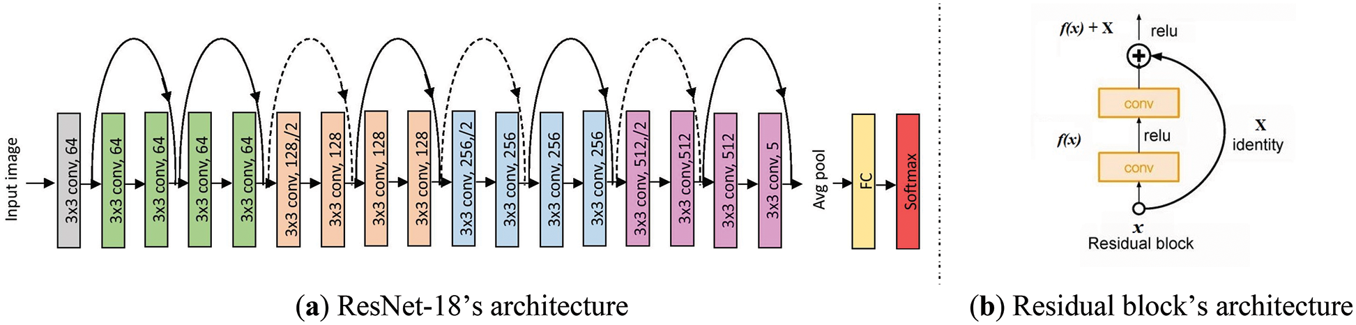
Figure 1: Architectures of ResNet-18 and residual block

DenseNet’s architecture is shown in reference [43]. It has a similar residual block as ResNet. The difference is that each layer in the dense block is feed-forward connected to all subsequent layers. For each layer, features of all preceding layers are inputs, and their outputs are inputs to all subsequent layers. DenseNet has fewer parameters than ResNet because feature reuse is enhanced.

The architectures of EfficientNet-B0 and mobile block (MB) are shown in reference [44]. The model includes nine stages, while stages 1–8 consist of the MBs. Every two MB has a residual block. In addition, a SE structure [24] is included in the MB to enhance channel attention.

The architecture of EfficientNetV2-S can be found in reference [13]. It is similar to that of EfficientNet-B0. However, an architecture search changes the scale ratio of MBs.

3.2 Method’s Framework

The proposed method’s framework is shown in Fig. 2. The method pipeline consists of two steps. In Step 1, the pre-trained models on ImageNet 2012 are retrained on RSI datasets by transfer learning strategies. Afterwards, in Step 2, the weight files from transfer-learned models are inherited and the models are fine-trained on RSI datasets. The biggest difference between Step 1 and Step 2 is the DA strategy. More details are presented in Sections 3.3 and 3.4.

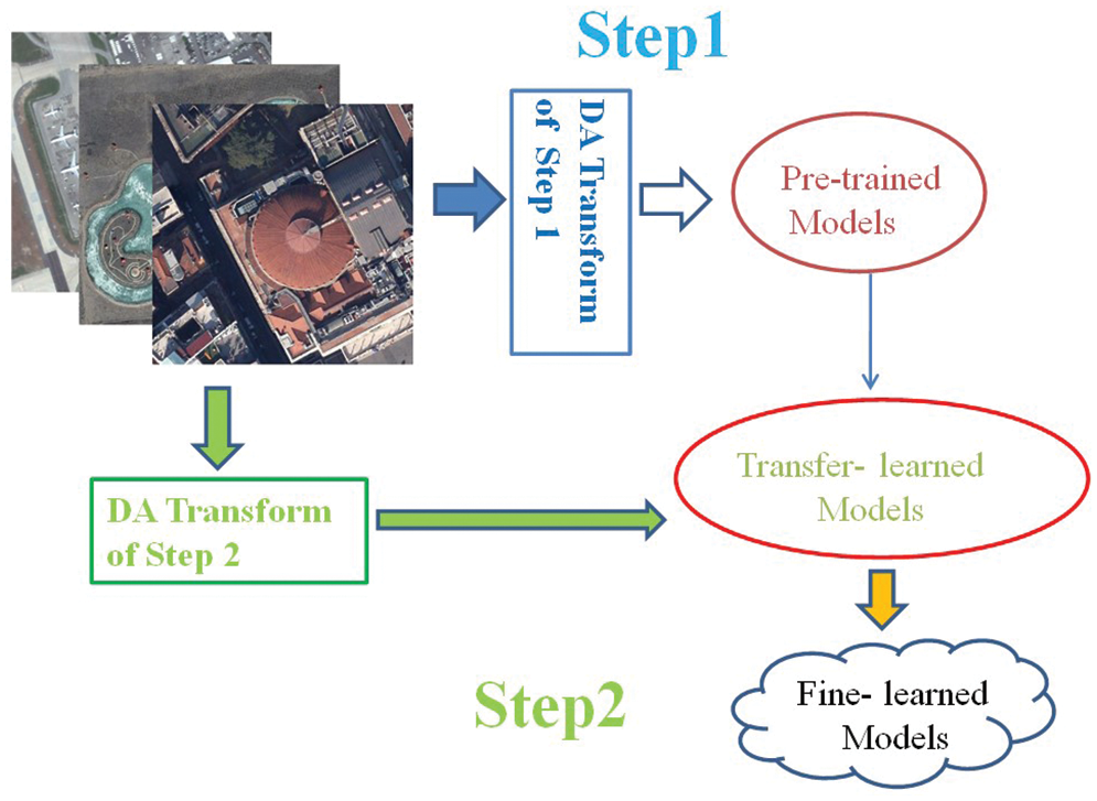
Figure 2: The proposed method’s framework

3.3 Algorithm

The algorithm of the FST-CNN is shown in Algorithm 1. In detail, three hyper-parameters are crucial to implement. Firstly, the Step 1 training epoch is 120, while the 180 epochs of Step 1 are only used on the smaller dataset. The model needs more samples from small datasets to achieve convergence. Secondly, the size of the training image transformed by the RSC is 1762. Extensive experiments confirmed that the empirical resolution can properly solve the data distribution shift [37]. Thirdly, the initial learning rate (LR) is 0.0001 for Step 1 and 0.00001 for Step 2, both with cosine decay. Commonly, a smaller LR has a smoother fitting curve for transfer learning strategies.

Additionally, other hyper-parameters are similar to previous studies. The batch size is 30. The testing resolution is 2562. The accuracy is the best result of Step 2, and the training epoch is empirical 240.

3.4 Data Augmentation

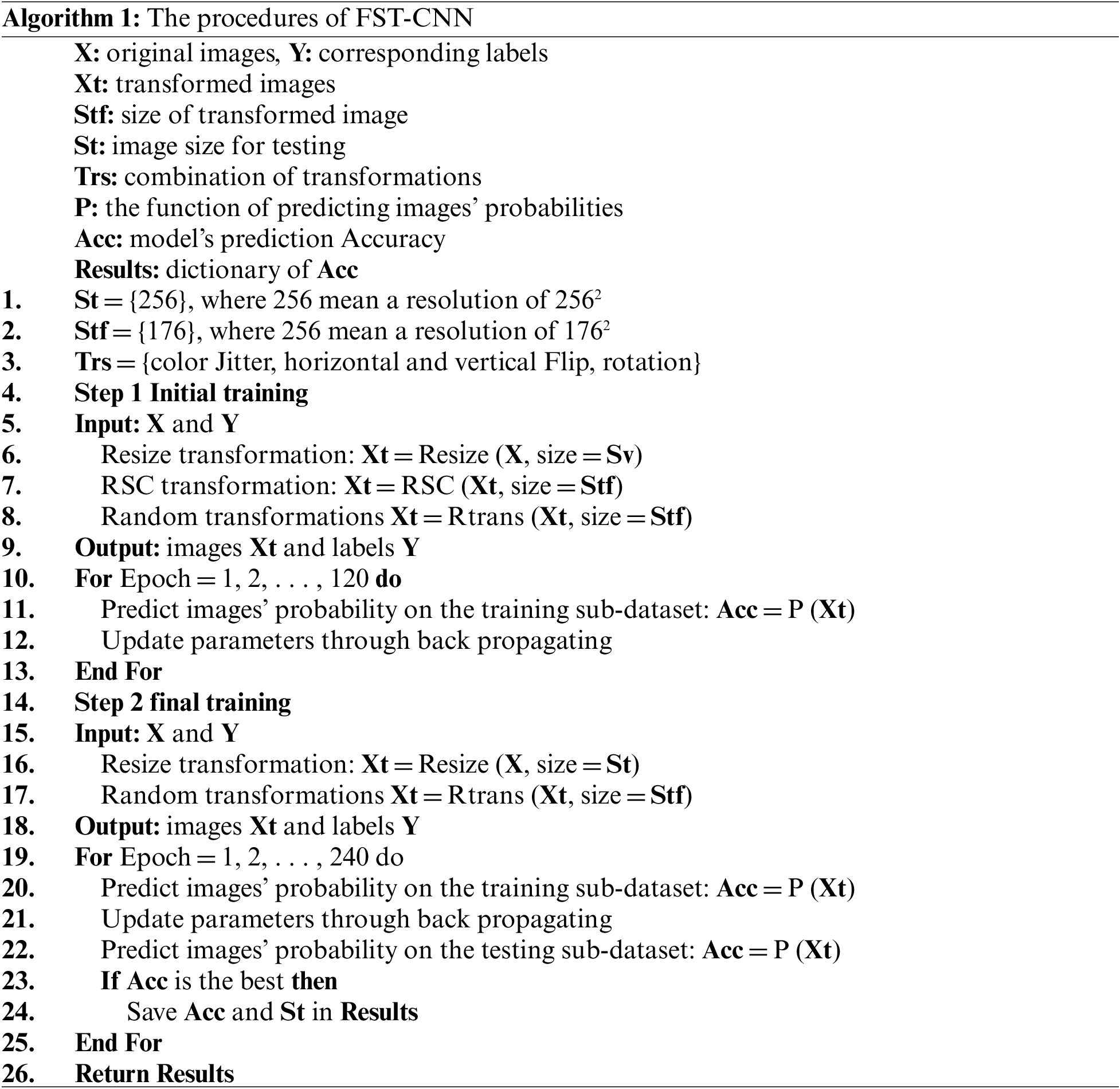
The DA in this study employs an understandable strategy that consists of six kinds of image transformations in a cascade combination. That is, the resize is followed by the RSC, and then there is the color jitter, horizontal flip, vertical flip, and rotation in turn. However, the RSC is excluded from Step 2. DA is implemented via the default code in the PyTorch libraries.

3.5 Dataset and Division

There are two RSI datasets widely used as benchmarks in previous studies, i.e., the Aerial Image Dataset (AID) and the Northwestern Polytechnic University Remote Sensing Image Scene Classification 45 Dataset (NWPU45D). The details about the two datasets can be found in reference [13]. Samples of some typical subsets in AID and NWPU45D are shown in Fig. 3.

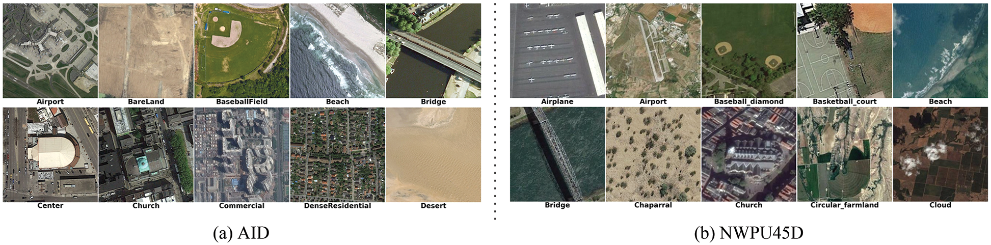
Figure 3: Typical samples in AID and NWPU45D

The training ratios of the two datasets are the same as in the previous studies, i.e., 20% and 50% for AID and 10% and 20% for NWPU45D. The training and testing subsets are also chosen at random.

3.6 Evaluation Criteria

In previous studies, the overall accuracy (OA) and confusion matrix were commonly used as criteria for performance evaluation. The definition of “confusion matrix” can be found in reference [13]. The OA is as described in Eq. (1):

OA=NcNt(1)

where OA is defined as the total number of accurately classified samples (Nc) divided by the total number of tested samples (Nt).

3.7 Hardware and Software Environments

The experiments were performed on four personal computers equipped with a single RTX 2060 GPU. PyTorch 1.11.0 is installed on Windows 10. All the models were initialized by the pre-trained weights file on ImageNet2012 in PyTorch. All the experimental results were averaged over three runs.

4  Results

4.1 Fitting Curves

The fitting curves of AID at a training ratio of 20% are shown in Fig. 4. As shown on the top of Fig. 4, it is clear that all five CNN models (i.e., the VGGNet-16, GoogLenet, DenseNet-121, ResNet-50, and EfficientNet-B0) achieve smooth fitting curves at training step 1. In detail, the accuracy curves show a fast fitting speed at the beginning 50 epochs. Afterwards, the convergent speed slows. This phenomenon is classical in transfer learning strategies.

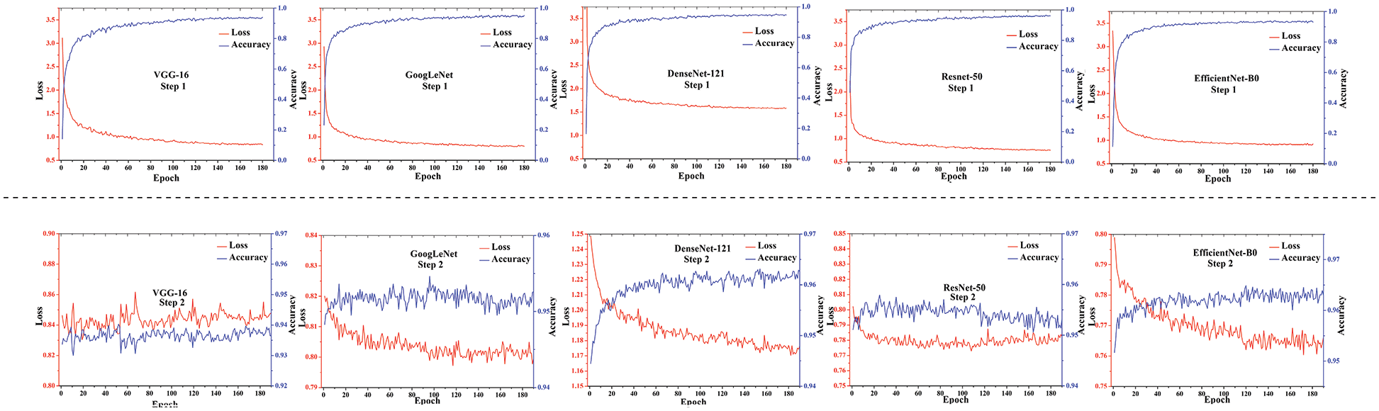
Figure 4: Fitting curves of AID at a 20% training ratio

As shown at the bottom of Fig. 4, all five models achieve a distinct accuracy lift, while the yields are slightly different. In detail, the lift amplitude is more obvious for DenseNet121 and EfficientNet-B0. Nonetheless, all five models show a consistent accuracy enhancement of 1.0%–1.6% after the data distribution shifting introduced by DA is corrected. These results may indicate that all the previous studies achieved suboptimal performance due to a lack of fine training.

4.2 OA Results for AID

The OA results of different methods on AID are shown in Table 1. As shown in Table 1, there are seventeen methods and thirty models included. The OA results in black from models trained by the FST-CNN algorithm are set as a baseline benchmark. The OA result in red means below the baseline, while green means above the baseline. The “None” means that no relevant results are presented in the literature.

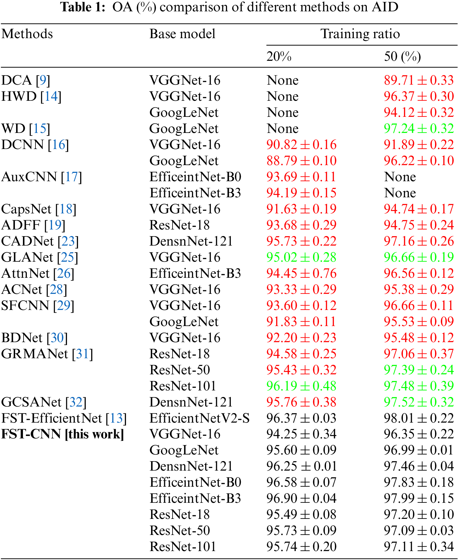
In detail, a maximal OA gap of 6.64% is found in the DCA method, which employs the VGGNet-16 architecture. Meanwhile, a similar gap of 2.87% is found in the DCNN method, which employs the GoogLeNet architecture. More specifically, only three of these seventeen methods have performance near or slightly beyond baseline results. However, the WD method only employs a smaller testing ratio of 30%, which makes its result doubtful. The GCSANet method also shows a very close result to the baseline when considering the error. The GLANet does show an improvement on the VGGNet-16 model. However, the VGGNet-16 architecture is out of fashion. The GRMANet results may indicate that the introduced GRU sequential architecture has the potential to boost model performance.

In any case, these true existence results show that the previous CNN-based approaches for RSI-SC have a systemic problem. This suboptimal performance issue across different methods and CNN-based architectures is supported by good empirical evidence. It reveals that a cognitive consistency bias has existed for over a half-decade.

4.3 OA Results for NWPU45D

The OA results of different methods on NWPU45D are shown in Table 2. There are sixteen methods and thirty base models included in Table 2. The OA results are illustrated by the same rule as Table 1.

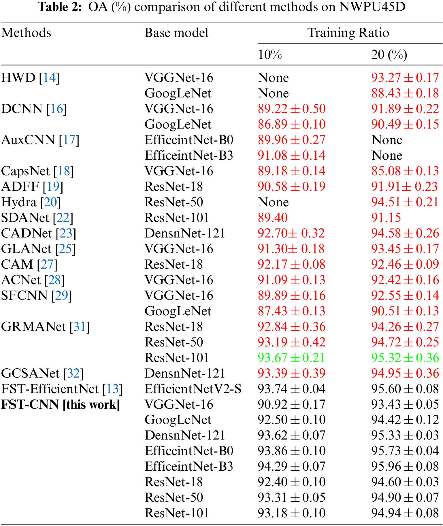
In detail, a maximal OA gap of 8.35% is found in the CapsNet method, which employs the VGGNet-16 architecture. Meanwhile, a similar gap of 5.99% is found in the HWD method, which employs the GoogLeNet architecture. More specifically, only one of these sixteen methods achieves performance beyond baseline results. The GRMANet method shows an acceptable improvement to the baseline on NWPU45D. It may indicate that sequential features extracted by CNN can do more than expected.

As a short conclusion, the OA results on AID and NWPU45D do show a consistent suboptimal performance in the previous studies for RSI-SC. Although different roadmaps have been employed, the final result is that “sample is the best.” The simple FST-CNN algorithm employs a traditional transfer learning strategy that overwhelms the other methods. These results demonstrate that there is a big chance to reshape the patterns for RSI-SC.

4.4 Confusion Matrixes of AID

The confusion matrix of AID at a 50% training ratio is shown in Fig. 5. It is the result of EfficeintNet-B3 being trained by the FST-CNN. There are 12 subclasses, including the airport, basketball field, beach, farmland, forest, parking, playground, pond, port, railway station, stadium, and viaduct, with an OA of 100%. Besides, there are three subclasses with an OA above 98%. The confusion mainly occurs in the subclasses, including center, park, resort, and school. In detail, the resort is at the lowest OA of 90%, while the square is at a lower 92%. This confusion result is consistent with other previous studies, although its OA is higher. It reveals that the performance gap between different CNN architectures is primarily due to their representation abilities.

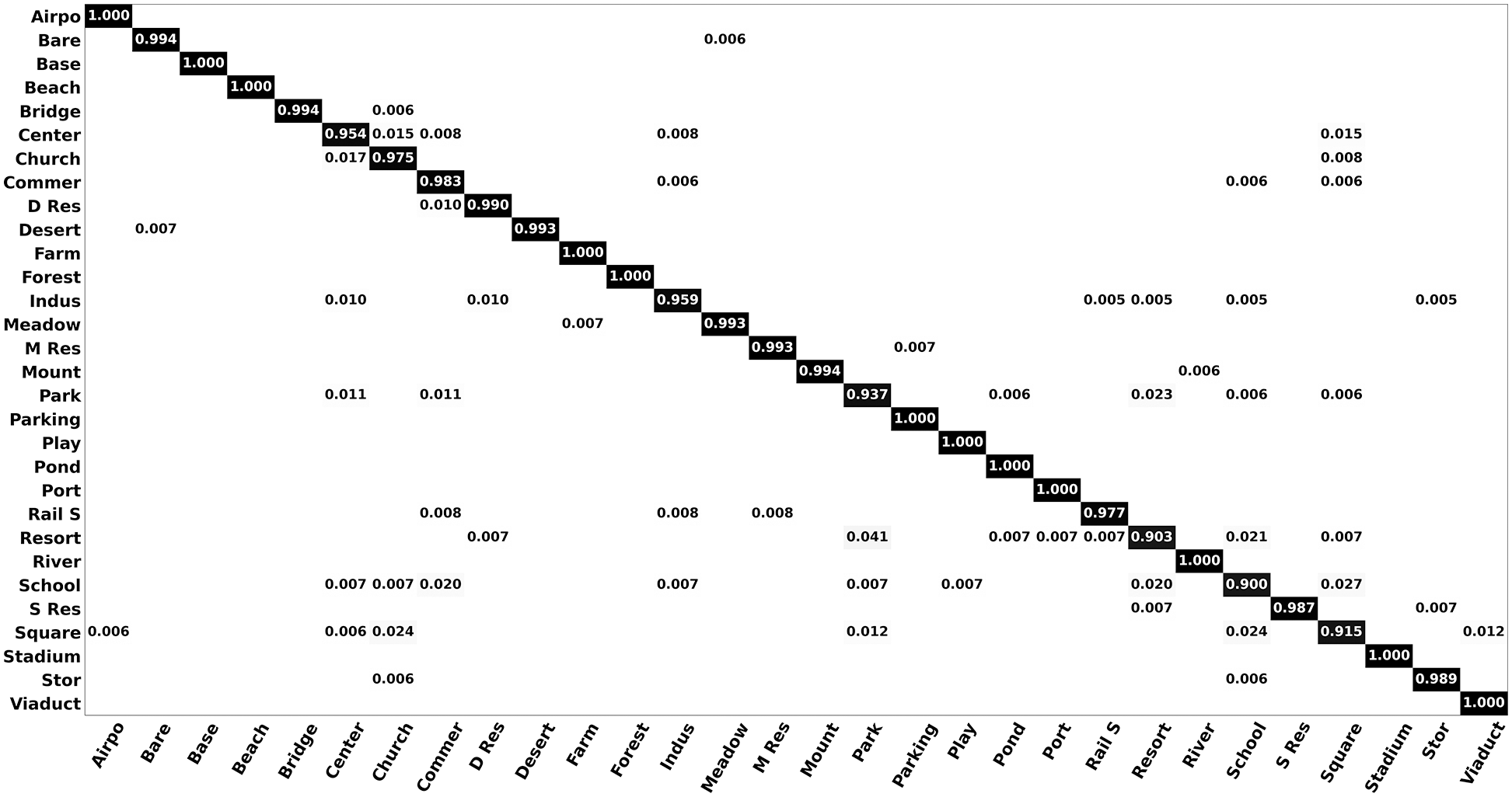
Figure 5: Confusion matrix of AID at a 50% training ratio

4.5 Confusion Matrixes of NWPU45D

The confusion matrix of NWPU45D at 20% training ratios is shown in Fig. 6. It is the result of EfficeintNet-B3 being trained by the FST-CNN. There are five subclasses, including the chaparral, harbor, sea ice, ship, and snow berg, with an OA of 100%. There are 30 subclasses with an OA above 95%. Besides, the confusion mainly occurs in the subclasses, including commercial area, dense residential area, industrial area, island, lake, medium residential, railway station, roundabout, snow berg, and wetland, with an OA below 95% but above 90%. Confusion is most prevalent in the church and palace, which have an OA of less than 90%. It reveals that the covariate shift in these two subclasses is more significant. The confusion results are consistent with other prior studies. It is generally agreed that the difference in interclass in NWPU45D is greater than AID. Firstly, the total number of samples in NWPU45D is three times that of AID. Secondly, the image’s resolution in NWPU45D is only 2562 compared to AID’s 6002.

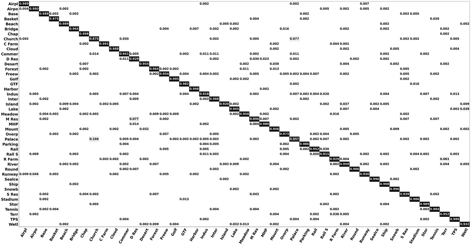
Figure 6: Confusion matrix of NWPU45D at a 20% training ratio

In brief, the results demonstrate that the FST-CNN algorithm significantly boosts the model’s performance.

4.6 Attention Maps

Attention maps generated by the GradCAM algorithm [45] are shown in Fig. 7. The brighter areas indicate more discernment information. As shown in Fig. 7a, the airport scene is correctly classified by all five CNN models. As shown in Fig. 7b, the church scene is obviously misclassified by VGGNet-16 due to the similarity between subclasses. The EfficientNet-B0 should have better discernment due to the SE attention structure. However, the clue was not clear in previous studies. The results do prove that most of the previous studies achieved suboptimal performance due to improper training procedures.

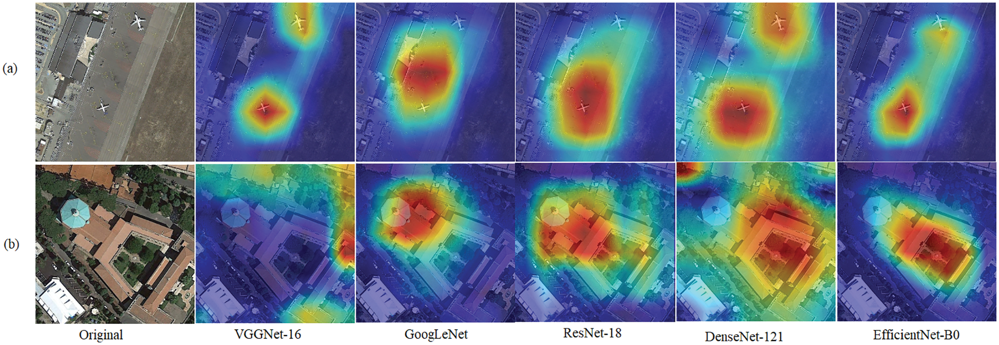
Figure 7: Original scene images and attention maps derived from Grad-CAM

4.7 Ablation Study

In this section, the DA strategy of Step 2 in the FST-CNN algorithm is used as the baseline to evaluate the effectiveness of RSC, LS, and fine-training on different CNN models for RSI-SC. That is, the baseline’s DA strategy excludes RSC and LS, while fine-training (i.e., the Step 2 train procedure) is employed for all tests. The experiments are tested on AID at a training ratio of 20%. The ablation studies’ results are shown in Table 3.

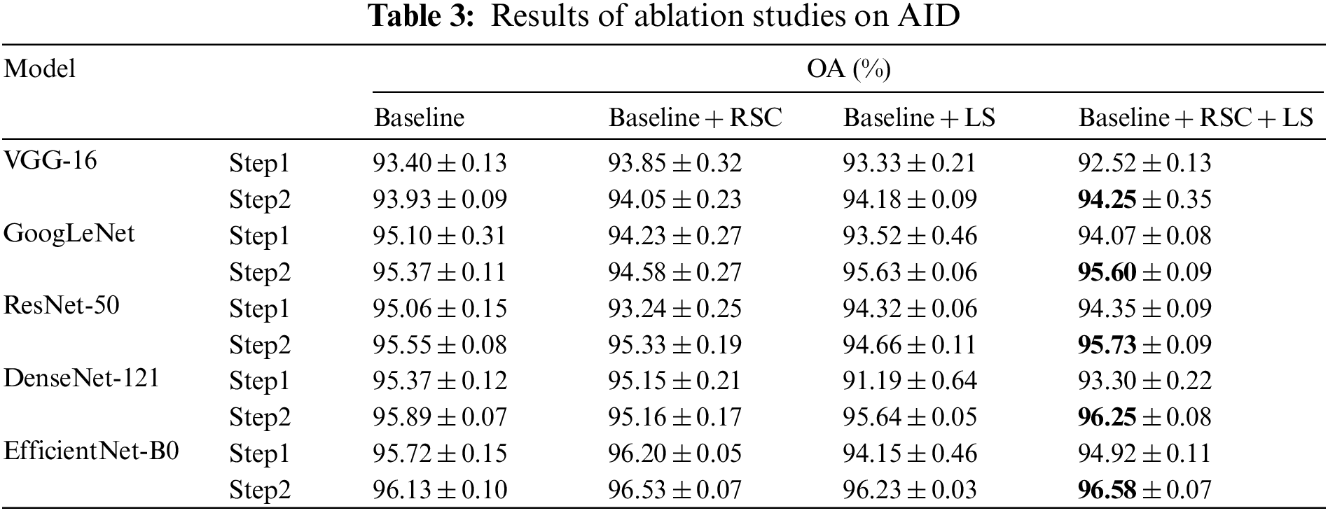
As shown in column “Baseline,” the fine-training procedure boosts all five models’ performance by a 0.4% to 0.5% increase in OA. This result reveals that the baseline DA strategy, which only consists of classic geometric and color transforms, also introduces a data distribution shift to the dataset. As shown in the column “Baseline + RSC,” the shift also exists, but the intensity is different across models. As shown in the column “Baseline + LS,” the shift intensity varies more across models. However, as shown in the column “Baseline + RSC + LS,” the fine-training procedure boosts all five models’ performance by a more noticeable 1.5% to 2.9% increase in OA.

In general, the results demonstrate that the data distribution shift introduced by DA truly exists. The ignore of the problem brought out the consistent suboptimal performance in the previous literature. However, the problem can be well handled in a cost-controlled way, just like the FST-CNN algorithm does.

5  Discussions

Feature extraction is a core skill for ML-based algorithms. However, these feature-reliance practices are quite different for DL methods. The results in this work demonstrate that the CNN model’s performance for RSI-SC cannot be improved by simple stacking features. That is, the features automatically extracted by the algorithms are very different from the handcrafted ones. In other words, those feature fusion strategies do not significantly boost the model’s performance as expected. Meanwhile, the benefit of stacking models is not proportional to the number of models. The results of the Hydra ensemble show that hardware costs will outweigh the benefits when the GPU budget is not well controlled.

Moreover, DA techniques like the RSC seem to be a cheaper option for CNN-based methods to achieve more multi-scale features if the data distribution shift is well handled. DA techniques are usually implemented on the CPU, so the GPU cost is more controllable. Meanwhile, the training images’ resolution generated by the RSC is commonly smaller than the original ones. Its training time is less expensive.

However, the results in this work prove that the previous studies paid more attention to the model’s architecture, feature extraction, and object function optimization. The training optimization strategies have been long ignored, so all the previous ones have achieved suboptimal results like an under-fitting problem. This problem has created a dilemma because it is difficult to evaluate the value of previous studies. It is time to double-check these methods.

6  Conclusions

The CNN-based algorithm is dominant in the current studies on interpreting RSI. However, it appears that training optimization strategies have received less attention in relevant research.

To evaluate this problem, the author proposes a novel training algorithm named FST-CNN. It employs a routine transfer learning strategy coupled with routine DA procedures. Afterward, to verify the algorithm’s effectiveness, 20 methods from previous studies are included in a performance comparison. In total, there are six classic models, and 30 architectures are involved and investigated. In detail, the same model architecture trained by the FST-CNN algorithm on the same datasets serves as the evaluation baseline.

The results reveal a real predicament in the previous studies for RSI-SC. That is, there is clear evidence of systemic suboptimal performance in the previous literature. In other words, most of the CNN-based methods proposed in the previous studies show a consistent mistake, which has made the model’s accuracy lower than its potential value. The most important reason seems to be the inappropriate training strategy and the data distribution shift introduced by DA.

Meanwhile, all those complex roadmaps, e.g., deep feature fusion, model combination, model ensembles, and human feature engineering, are not as effective as expected. More than that, most of the performance evaluation was conducted based on an inaccurate, suboptimal, and unfair result. It has made most of the previous studies’ research findings questionable to some extent.

However, all these confusing results also exactly demonstrate the effectiveness of FST-CNN. This novel algorithm is model-agnostic and can be employed on any image classification model to potentially boost performance. In addition, the results also show that a standardized training strategy is indeed very meaningful for the research tasks of the RSI-SC.

Anyhow, some ideas truly show the possibility of boosting CNN’s performance further, e.g., the sequential deep features and the attention blocks. Additionally, the model’s performance seems to be saturated, even though the training samples are doubled in the Step 2 process of the FST-CNN algorithm. It seems to come from the architecture’s heterogeneity. We will investigate all similar questions thoroughly in the future.

Acknowledgement: Thanks to the anonymous reviewers for their valuable suggestions.

Funding Statement: Hunan University of Arts and Science provided doctoral research funding for this study (grant number 16BSQD23). Fund of Geography Subject ([2022] 351) also provided funding.

Conflicts of Interest: The author declares that he has no conflicts of interest to report regarding the present study.

References

1. A. E. Maxwell, T. A. Warner and F. Fang, “Implementation of machine-learning classification in remote sensing: An applied review,” International Journal of Remote Sensing, vol. 39, no. 9, pp. 2784–2817, 2018. [Google Scholar]

2. J. Cai, J. Luo, S. Wang and S. Yang, “Feature selection in machine learning: A new perspective,” Neurocomputing, vol. 300, pp. 70–79, 2018. [Google Scholar]

3. P. Wang, B. Bayram and E. Sertel, “ A comprehensive review on deep learning based remote sensing image super-resolution methods,” Earth-Science Reviews, vol. 232, pp. 104110, 2022. [Google Scholar]

4. K. Saranya and K. Selva Bhuvaneswari, “Semantic annotation of land cover remote sensing images using fuzzy CNN,” Intelligent Automation & Soft Computing, vol. 33, no. 1, pp. 399–414, 2022. [Google Scholar]

5. J. Luo, J. Zeng, J. Fu, X. Fu and L. Leng, “Aircraft target recognition in remote sensing images based on saliency maps and invariant moments,” in Proc. ICGG, Milan, MI, Italy, pp. 1358–1365, 2018. [Google Scholar]

6. D. Wu, C. J. Zhang, L. Ji, R. Ran, H. Y. Wu et al., “Forest fire recognition based on feature extraction from multi-view images,” Traitement du Signal, vol. 38, no. 3, pp. 775–783, 2021. [Google Scholar]

7. A. E. Maxwell, T. A. Warner and L. A. Guillén, “Accuracy assessment in convolutional neural network-based deep learning remote sensing studies—Part 1: Literature review,” Remote Sensing, vol. 13, no. 13, pp. 2450, 2021. [Google Scholar]

8. F. Hu, G. S. Xia, J. Hu and L. Zhang, “Transferring deep convolutional neural networks for the scene classification of high-resolution remote sensing imagery,” Remote Sensing, vol. 7, no. 11, pp. 14680–14707, 2015. [Google Scholar]

9. S. Chaib, H. Liu, Y. Gu and H. Yao, “Deep feature fusion for VHR remote sensing scene classification,” IEEE Transactions on Geoscience and Remote Sensing, vol. 55, no. 8, pp. 4775–4784, 2017. [Google Scholar]

10. Y. Ge, Y. Tang, S. Jiang, L. Leng, S. Xu et al., “Region-based cascade pooling of convolutional features for HRRS image retrieval,” Remote Sensing Letters, vol. 9, no. 10, pp. 1002–1010, 2018. [Google Scholar]

11. Z. Liu, H. Mao, C. Y. Wu, C. Feichtenhofer, T. Darrell et al., “A convnet for the 2020s,” in Proc. CVPR, New Orleans, LA, USA, pp. 11976–11986, 2022. [Google Scholar]

12. W. Khan, K. Raj, T. Kumar, A. M. Roy and B. Luo, “Introducing urdu digits dataset with demonstration of an efficient and robust noisy decoder-based pseudo example generator,” Symmetry, vol. 14, no. 10, pp. 1976, 2022. [Google Scholar]

13. H. Song, “A more efficient approach for remote sensing image classification,” Computers, Materials & Continua, vol. 74, no. 3, pp. 5741–5756, 2023. [Google Scholar]

14. Y. Liu, C. Y. Suen, Y. Liu and L. Ding, “Scene classification using hierarchical Wasserstein CNN,” IEEE Transactions on Geoscience and Remote Sensing, vol. 57, no. 5, pp. 2494–2509, 2018. [Google Scholar]

15. Y. Liu, Y. Liu and L. Ding, “Scene classification by coupling convolutional neural networks with wasserstein distance,” IEEE Geoscience and Remote Sensing Letters, vol. 16, no. 5, pp. 722–726, 2018. [Google Scholar]

16. G. Cheng, C. Yang, X. Yao, L. Guo and J. Han, “When deep learning meets metric learning: Remote sensing image scene classification via learning discriminative CNNs,” IEEE Transactions on Geoscience and Remote Sensing, vol. 56, no. 5, pp. 2811–2821, 2018. [Google Scholar]

17. Y. Bazi, M. M. A. Rahhal, H. Alhichri and N. Alajlan, “Simple yet effective fine-tuning of deep CNNs using an auxiliary classification loss for remote sensing scene classification,” Remote Sensing Letters, vol. 11, no. 24, pp. 2908, 2019. [Google Scholar]

18. W. Zhang, P. Tang and L. Zhao, “Remote sensing image scene classification using CNN-CapsNet,” Remote Sensing, vol. 11, no. 5, pp. 494, 2019. [Google Scholar]

19. R. Zhu, L. Yan, N. Mo and Y. Liu, “Attention-based deep feature fusion for the scene classification of high-resolution remote sensing images,” Remote Sensing, vol. 11, no. 17, pp. 1996, 2019. [Google Scholar]

20. R. Minetto, M. P. Segundo and S. Sarkar, “Hydra: An ensemble of convolutional neural networks for geospatial land classification,” IEEE Transactions on Geoscience and Remote Sensing, vol. 57, no. 9, pp. 6530–6541, 2019. [Google Scholar]

21. A. Dosovitskiy, L. Beyer, A. Kolesnikov, D. Weissenborn, X. Zhai et al., “An image is worth 16×16 words: Transformers for image recognition at scale,” 2021. [online]. Available: https://arxiv.org/abs/2010.11929 [Google Scholar]

22. D. Guo, Y. Xia and X. Luo, “Scene classification of remote sensing images based on saliency dual attention residual network,” IEEE Access, vol. 8, pp. 6344–6357, 2020. [Google Scholar]

23. W. Tong, W. Chen, W. Han, X. Li and L. Wang, “Channel attention based DenseNet network for remote sensing image scene classification,” IEEE Journal of Selected Topics in Applied Earth Observations and Remote Sensing, vol. 13, pp. 4121–4132, 2020. [Google Scholar]

24. J. Hu, L. Shen and G. Sun, “Squeeze-and-excitation networks,” in Proc. CVPR, Salt Lake City, UT, USA, pp. 7132–7141, 2018. [Google Scholar]

25. Y. Guo, J. Ji, X. Lu, H. Huo, T. Fang et al., “Global-local attention network for aerial scene classification,” IEEE Access, vol. 7, pp. 67200–67212, 2019. [Google Scholar]

26. H. Alhichri, A. S. Alswayed, Y. Bazi, N. Ammour and N. A. Alajlan, “Classification of remote sensing images using EfficientNet-b3 CNN model with attention,” IEEE Access, vol. 9, pp. 14078–14094, 2021. [Google Scholar]

27. J. Li, D. Lin, Y. Wang, G. Xu, Y. Zhang et al., “Deep discriminative representation learning with attention map for scene classification,” Remote Sensing, vol. 12, no. 9, pp. 1366, 2020. [Google Scholar]

28. X. Tang, Q. Ma, X. Zhang, F. Liu, J. Ma et al., “Attention consistent network for remote sensing scene classification,” IEEE Journal of Selected Topics in Applied Earth Observations and Remote Sensing, vol. 14, pp. 2030–2045, 2021. [Google Scholar]

29. J. Xie, N. He, L. Fang and A. Plaza, “Scale-free convolutional neural network for remote sensing scene classification,” IEEE Transactions on Geoscience and Remote Sensing, vol. 57, no. 9, pp. 6916–6928, 2019. [Google Scholar]

30. H. Sun, S. Li, X. Zheng and X. Lu, “Remote sensing scene classification by gated bidirectional network,” IEEE Transactions on Geoscience and Remote Sensing, vol. 58, no. 1, pp. 82–96, 2020. [Google Scholar]

31. B. Li, Y. Guo, J. Yang, L. Wang, Y. Wang et al., “Gated recurrent multiattention network for VHR remote sensing image classification,” IEEE Transactions on Geoscience and Remote Sensing, vol. 60, pp. 5606113, 2022. [Google Scholar]

32. W. Chen, S. Ouyang, W. Tong, X. Li, X. Zheng et al., “GCSANet: A global context spatial attention deep learning network for remote sensing scene classification,” IEEE Journal of Selected Topics in Applied Earth Observations and Remote Sensing, vol. 15, pp. 1150–1162, 2022. [Google Scholar]

33. J. Howard, “Training imagenet in 3 hours for 25 minutes,” 2018. [online]. Available: https://www.fast.ai/2018/04/30/dawnbench-fastai/ [Google Scholar]

34. E. Hoffer, B. Weinstein, I. Hubara, T. Ben-Nun and T. Hoefler, “Mix & match: Training convnets with mixed image sizes for improved accuracy, speed and scale resiliency,” 2019. [online]. Available: https://arxiv.org/abs/1908.08986 [Google Scholar]

35. M. Tan and Q. V. Le, “Efficientnetv2: Smaller models and faster training,” 2021. [online]. Available: https://arxiv.org/abs/2104.00298v3 [Google Scholar]

36. H. Touvron, A. Vedaldi, M. Douze and H. Jégou, “Fixing the train-test resolution discrepancy,” 2020. [online]. Available: https://arxiv.org/abs/2003.08237v1 [Google Scholar]

37. H. Song, “FST-Efficientnetv2: Exceptional image classification for remote sensing,” Computer Systems Science and Engineering, 2023. https://doi.org/10.32604/csse.2023.038429 [Google Scholar] [CrossRef]

38. I. Loshchilov and F. Hutter, “Decoupled weight decay regularization,” 2019. [online]. Available: https://arxiv.org/abs/1711.05101 [Google Scholar]

39. C. Szegedy, V. Vanhoucke, S. Ioffe, J. Shlens and Z. Wojna, “Rethinking the inception architecture for computer vision,” 2015. [online]. Available: https://arxiv.org/abs/1512.00567 [Google Scholar]

40. K. Simonyan and A. Zisserman, “Very deep convolutional networks for large-scale image recognition,” 2015. [online]. Available: https://arxiv.org/abs/1409.1556 [Google Scholar]

41. C. Szegedy, W. Liu, Y. Jia, P. Sermanet, S. Reed et al., “Going deeper with convolutions,” in Proc. CVPR, Salt Boston, MA, USA, pp. 1–9, 2015. [Google Scholar]

42. K. He, X. Zhang, S. Ren and J. Sun, “Deep residual learning for image recognition,” in Proc. CVPR, Las Vegas, NV, USA, pp. 770–778, 2016. [Google Scholar]

43. G. Huang, Z. Liu, L. V. D. Maaten and K. Q. Weinberger, “Densely connected convolutional networks,” in Proc. CVPR, Honolulu, HI, USA, pp. 4700–4708, 2017. [Google Scholar]

44. M. Tan and Q. V. Le, “Efficientnet: Rethinking model scaling for convolutional neural networks,” 2020. [online]. Available: https://arxiv.org/abs/1905.11946 [Google Scholar]

45. R. R. Selvaraju, M. Cogswell, A. Das, R. Vedantam, D. Parikh et al., “Grad-cam: Visual explanations from deep networks via gradient-based localization,” in Proc. ICCV, Venice, PD, Italy, pp. 618–626, 2017. [Google Scholar]