Reconfigurable Sensing Time in Cooperative Cognitive Network Using Machine Learning

1  Introduction

Investigation of the radio spectrum reveals that portions of the allocated heavily radio spectrum to multiple licensed or primary users (PU) are not occupied uniformly. Few of the frequency bands are massively utilized, some are void, and the others are filled partially by the PU. A spectrum hole is part of a frequency band assigned to the PUs but not utilized at a particular time and specified geographical location. Cognitive radio (CR) intelligently keeps itself aware of the surrounding radio environment. The CR senses the PU channels and adapts the internal states such as carrier frequency, modulation strategy, and transmitting power to provide reliable communication relevant to statistical variations in the incoming radio frequency stimuli [1,2]. In the cognitive radio network (CRN), secondary users (SUs) perform spectrum sensing to dynamically access the PUs channel when the PU is not active [3,4]. The wireless channel properties of the multipath fading and shadowing create ambiguities in the individual SU sensing. Thus, to tackle these challenges, it is more appropriate to utilize cooperative spectrum sensing (CSS) [3–7]. In the centralized CSS, a central base station, such as a fusion center (FC) receives sensing information from the SUs in the hard or soft modes for the final decision about the presence and absence of PU [8,9]. The hard decision fusion (HDF) often employs logical AND, logical OR, and majority voting schemes [10–12]. In the soft decision fusion (SDF), such as maximum gain combining (MGC), equal gain combining (EGC), and Kullback-Leibler (KL) divergence schemes, SUs forward soft sensing reports to the FC to make the final decision [13–16]. Influenced by certain motives, malicious users (MUs) may intrude into the CSS networks. The security threats and camouflage of CSS from the MUs are investigated in [17–20]. In [12,21], the authors studied the optimization of detection and false alarm probabilities of the SUs employing particle swarm optimization (PSO) and genetic algorithm (GA). In [22], the problem of composing sensing duration is examined to maximize SUs throughput with a constraint on PUs protection. The work in [23] offers a unified framework for the reconfigurable wireless network that provides a comprehensive view of the method and strategies. Joint optimization of the individual channel parameters and sensing duration is performed in [24] to maximize SUs throughput with a constraint to minimize interference for the PUs. An optimal framework of the multichannel spectrum sensing for CRN is presented in [25]. The work in [26] investigates the sensing throughput with the design of optimal sensing time and power allocation that maximize the CRN throughput and maintain PUs quality of service (QoS).

Artificial intelligence (AI) techniques are considered competent to enhance the sensing capability of CR technology. Applications of AI in CRNs have been encouraged in the literature. The role and importance of learning in [27] exhibit a brief survey of AI and machine learning (ML) tools for CRs. In [28], the authors provided an overview of intelligent communication and illustrated the revolution from cognition to AI. An adaptive scheme is proposed in [29] that optimizes the sensing period of the CRN using multi-objective GA. In [30], AI-based abnormality detection techniques are presented in CR to enable the ML models for data dimensionality and sampling rates. As the concept of the cognition cycle (CC) is the foundational element of CR, which provides context recognition and intelligence to unlicensed users, therefore, the work in [31] realizes the concept of reinforcement learning (RL) to achieve CC. The work in [32] proposed ML-based modulation and recognition algorithm at the CR receivers to monitor real-time wideband spectral usage. The traditional spectrum sensing techniques consume considerable time and energy in sensing the PU. Therefore, hierarchical spectrum sensing schemes based on convolutional neural networks (CNNs) and deep learning are investigated in [33–35]. A cluster-based CSS solution is proposed in [36,37], where clustering is assumed to be performed by the upper layer.

The increased number of sensing samples leads to better sensing accuracy but with related challenges, such as lower data transmission time yielding low throughput and more energy consumption. Conversely, an optimal number of sensing samples in an individual or CSS environment may increase the throughput, lower the energy consumption, and guarantee the sensing performance, with minimum error probabilities. The studies in [24–26] solve a similar problem employing multi-channel detection without considering the AI techniques. Contrarily, the proposed scheme uses AI techniques to reconfigure the sensing time. In this paper, we utilize the fine-k-nearest neighbor (FKNN) algorithm to obtain optimal sensing samples bearing low false alarms and high detection probabilities yielding minimum sensing error. The main contributions of the paper are as follows:

•   A centralized CSS is examined while searching PU channel information. The individual users in the proposed work are assumed to be at distinct geographical positions encountering the PU channel differently, therefore, the system treats their sensing reports differently in the global decision.

•   A data set is established for the energy detector considering detection probability function under the additive white gaussian noise (AWGN) channel condition.

•   This work focuses on the FKNN to determine optimum sensing samples against the local sensing reports from the SUs at different positions.

•   Once the optimum number of sensing samples are determined using the FKNN algorithm, these samples are utilized for sensing PU channel and combined in the soft combination schemes such as MGC and EGC to make global decisions.

•   Extensive results of the energy consumption, channel throughput, and error probabilities are collected for the traditional and proposed soft combination schemes. These simulations confirmed improved sensing response with low energy consumption, high channel throughput, and minimum sensing error for the proposed FKNN based centralized CSS. The results are compared with conventional MGC, EGC, and Count fusion schemes based on fixed samples (FS), decision tree (DT) algorithms, and linear regression (LR).

The rest of the paper is categorized as follows. Section 2 presents the system model. In Section 3, the FKNN-based SDF scheme is discussed. Section 4 evaluates and compares the proposed and conventional schemes through extensive results. Finally, conclusive remarks are shown in Section 5.

2  System Model and Background

The system model assumes a CRN with M SUs, that opportunistically share the PU channel. SUs sense the presence or absence of the PU signal and decide the PU occupancy. A single PU channel is assumed for simplicity. The SUs follow an energy detector for local spectrum sensing.

In Fig. 1, the cognitive users report their soft energy observations to the FC to produce a suitable decision. The PU channel occupancy at the individual sensing users is referred to as H0 and H1. The H0 and H1 shows no activity (channel is available) and busy status (channel is occupied) by the PU observed at the jth user as

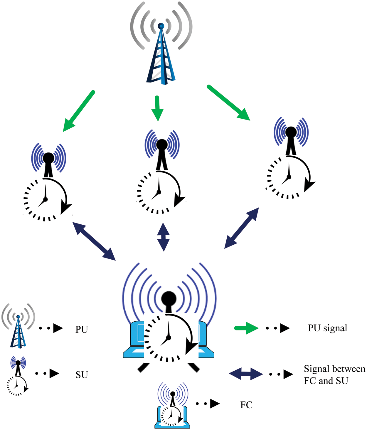
Figure 1: CSS with reconfigurable sensing time

{H0,xj(l)=vj(l)H1,xj(l)=gjc(l)+vj(l)},j∈{1,2,…,M},l∈{1,2,…,K}.(1)

Eq. (1) shows the channel gain gj between the primary and jth sensing user. c(l) is the PU signal in the lth slot that has zero mean and variance σc2. The vj(l) is the AWGN between the primary jth sensing user that has mean zero and variance σvj2. The sensing energy is Gaussian with enough sensing samples K=2Bτs for the H0 and H1 hypothesis. Here B is the bandwidth and τs is the sensing period. The observed energy based on H1 and H0 in Eq. (1) is represented as

Ej(i)={∑l=lili+K−1|vj(l)|2,H0∑l=lili+K−1|gjc(l)+vj(l)|2,H1},(2)

where K is the total number of sensing samples in each sensing period. In the case of a sufficiently larger K value, the soft energy reports of the users in Eq. (2) converge to the Gaussian random variable as

Ej∼{N(μ0=K,σ02=2K),H0N(μ1=K(ηj+1),σ12=2K(ηj+1)),H1}.(3)

In Eq. (3), ηj is jth sensing user channel signal-to-noise-ratios (SNRs), while (μ0,σ02) and (μ1,σ12) are mean and variances of the energy distribution when the H0 and H1 hypotheses are true.

The sensing users in Fig. 2 sense the channel during τs period and transmit the data in the T−τs when the channel is free by the licensee. The time slots are assumed to be synchronized. The channel in each of these slots is either of the two states H1 and H0. Therefore, the local sensing information will either represent a high or low energy signal during any sensing slot.

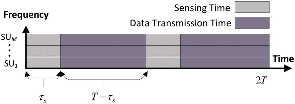
Figure 2: Sensing and data transmission time

The two scenarios that decide the PU channel status are independent and collaborative sensing. In the independent scenario, SU senses and makes a decision locally, to infer the PU channel availability. As the individual sensing reliability is affected due to various aspects in the wireless channel, therefore, to improve this, collaborative sensing is performed. Each SU in CSS reports its local decision to the FC to take the final decision. The SUs are assumed to take the decisions based on the soft energy collections. The FC informs back the cooperative users about its global decision. A dedicated control channel is assumed for transmission between the SUs and FC.

In CSS, the FC freely practices in soft or hard combination schemes. The commonly used soft combinations are MGC and EGC, while the hard combination schemes include the logical OR, logical AND, and majority voting. In this paper, FC combines local sensing reports using EGC, MGC, and count combinations. In EGC, FC deals with the individual user report equally and assigns similar sensing weights to each user-reported data, while the MGC distributes separate weights. The channel with high SNRs gets high sensing weight at the FC, and the one with low SNR values receives low sensing weight at the FC.

3  Reconfigurable Sensing Time and Channel Estimation

The proposed scheme is discussed in this section to find optimum sensing results that lead to minimum sensing error. This section first discusses the FKNN classifier. In the second part, optimum sensing samples using the FKNN algorithm for a given target SNRs, detection, and false alarm probabilities are determined. As the individual users are at different geographical positions, their sensing samples are also different. The throughput and sensing cost relation with the sample size is also discussed in this section.

3.1 Fine-k-Nearest Neighbor (FKNN)

Various linear and nonlinear classification algorithms are explored to choose an ML technique that works best in the given problem and, FKNN is found superior. The FKNN in Fig. 3 operates to find the shortest distance between data and evaluate the closest neighbors to the training data pattern. FKNN is more leisurely to implement in finding a solution to the problem. This technique classifies a new test data (feature vector) based on the distance of the new test data from multiple nearby neighbors. The FKNN generalizes the data referring to attributes of training samples, where the given query point finds several training instances closest to the query point. This classification is based on the majority voting to classify the objects. The FKNN is a simple algorithm that operates on the shortest distance of a query instance to the training sample.

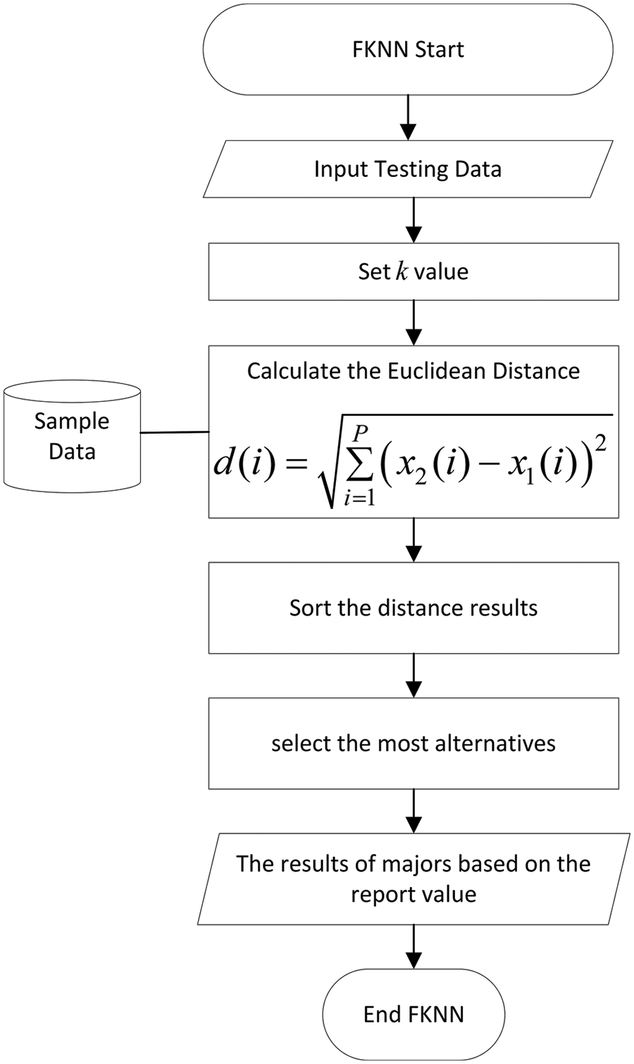
Figure 3: Working principle of the FKNN algorithm

For x1 as the sample data and x2 as the data test/testing data. The distance formed (d) using the k-nearest neighbor (KNN) is as

d(i)=∑i=1P(x2(i)−x1(i))2,(4)

where i is the data variable and P as the dimension of the data.

Proper selection of the KNN parameters depends on the data requirements. A high value k reduces the noise effect but drawing the line between classes becomes blurred. Therefore, the k value is selected after fine-tuning through cross-validation. The KNN classifier that effectively solves the given problem is the FKNN algorithm. The tuning parameters for the FKNN have a total neighbor of two. The distance metric in the FKNN is Euclidean distance. Similarly, the distance weights are equal, and the data standardization option is turned on.

3.2 Dataset for the FKNN to Reconfigure Optimal Sensing Time

This section shows the design procedure to construct the data set for the ML classifier. The soft energy statistics in Eq. (3) attain suitable sensing samples for a given detection, false alarm, and SNRs as

Pf=Q((β−μ0)(σ02))=Q((β−K)(2K)),(5)

Here Pf is the probability of false alarm, β is the threshold value. μ0 and σ02 are the mean and variance when H0 is true. Similarly, the result of detection probability Pd when the H1 is true is

Pd=Q((β−μ1)(σ12))=Q((β−K(ηj+1))(2K(ηj+1))),(6)

In Eq. (6), μ1 and σ12 are mean and variance for the jth when H1 is true with ηj as the SNRs. The FKNN finds the optimal number of sensing samples in this work using the probability of detection function. Therefore, expressing the detection probability in Eq. (6) in terms of the false alarm probability in the AWGN channel conditions leads to the following [7]

Pd=Q((2Q−1(Pf)−Kηj)(2(ηj+1))).(7)

The Q(.) and Q−1(.) are the complementary and inverse complementary distribution functions of the standard Gaussian. In Eq. (7), to find optimal sensing samples K for a given detection and false alarm probabilities needs the solution of a non-convex function, which is hard to get in real-time. Therefore, the result in Eq. (7) is employed to generate a data set and train the FKNN scheme compared with traditional methods. The trained model is finally used to estimate the value of optimal sensing samples that are employed in the throughput, sensing cost, and soft fusion combination schemes. The feature vector or example of a data point in the dataset is represented with a vector as

x=(ηj,Pf,K,Pd)(8)

This feature vector consists of SNRs ηj, false alarm probability Pf, detection probability Pd, and samples K. The detection probabilities are obtained for the different combinations of the SNRs, false alarms, and several samples to get the dataset. The FKNN model is trained using the (ηj,Pf,Pd) as input and Kj as the output feature. The FKKN estimates the reconfigurable sensing samples for the jth SU as

Kj=FKNN([PfPdηj])(9)

3.3 Throughput and Sensing Cost

The trained model is used to estimate the optimum sensing sample Kj based on the new values of SNRs, detection and false alarm requirements. A reconfiguration of the sensing parameters such as Kj results in increased throughput and reduce in sensing cost. The channel capacity formula is employed to measure the SUs throughput as

C=∑j=1M(Cj)=∑j=1M(B×log2⁡(1+ηj)).(10)

Here Cj is the channel capacity with channel bandwidth B. The throughput for an SU using Eq. (10) in a time slot T is given by:

H=∑j=1MHj=∑j=1M(Cj×(T−τj)).(11)

In Eq. (11), Hj is the jth user throughput with τj sensing time and (T−τj) as the data transmission duration. The result in Eq. (11) shows the throughput is linear dependent on the data transmission duration with fixed T. Therefore, for a fix T reduction in the sensing duration τj leads to a higher throughput. As τj=Kjfs has the sampling frequency fs as a fixed parameter. Therefore, higher sensing throughput is obtained by lowing the τj through reduced sensing samples Kj. In the non-configurable CRN, the parameter K is fixed, while the suggested re-configurable network estimates the optimum results Kj using the FKNN algorithm and varies based on the sensing environment. The energy spent in sensing is directly proportional to the sensing duration and is represented as

S(i)=∑j=1M(Ej(i)×τj),(12)

where, S(i) is the sensing energy consumed by the cooperative users in the ith sensing interval and Ej is the sensing energy spent by the jth user based on the reconfigured sensing samples Kj. The increase in Kj=τj×fs is expected to increase the sensing cost of the system in Eq. (12).

3.4 Global Decision Using Reconfigured Sensing Time

The FC combines soft energy reports of all SUs in the final decision. The famously soft and hard combination schemes used at the FC are the EGC, MGC, and majority voting schemes. The EGC method combines the soft information and assigns equal weight to each SU decision. This result is compared with the numerical set threshold to decide the spectrum as

GEGC(i)={H1:1M∑j=1M(Ej(i)×τj)≥(β)H0:otherwise.(13)

The cooperative detection and false alarm probabilities of the EGC scheme based on its global decision are

Pd_EGC=Pr{1M∑j=1M(Ej(i)×τj)≥(β)|H1},(14)

Pf_EGC=Pr{1M∑j=1M(Ej(i)×τj)≥(β)|H0}.(15)

In the MGC, each received signal branch is multiplied by a weight proportional to the branch gain. The branches with strong signals get amplification while the weak signals are attenuated with these weights. The FC with MGC scheme assigns higher weights to the decision of the SUs with higher SNR and low weights to the SUs with low SNR

GMGC(i)={H1:∑j=1M(wj×(Ej(i)×τj))≥(β)H0:otherwise,(16)

where wj=η(j)∑j=1Mη(j). The cooperative detection and false alarm probabilities of the MGC are measured based on the individual sensing reports as

Pd_MGC={∑j=1M(wj×(Ej(i)×τj))≥(β)|H1},(17)

Pf_MGC={∑j=1,M(wj×(Ej(i)×τj))≥(β)|H0}.(18)

A precise flow diagram in Fig. 4 shows the training and testing strategy of the FKNN-based hybrid scheme at the FC.

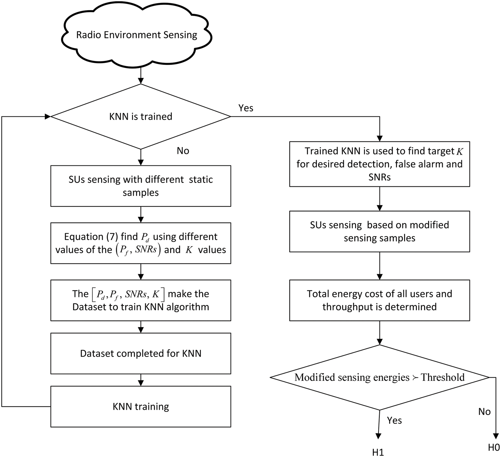
Figure 4: Flowchart of the proposed scheme

4  Numerical Evaluation and Discussions

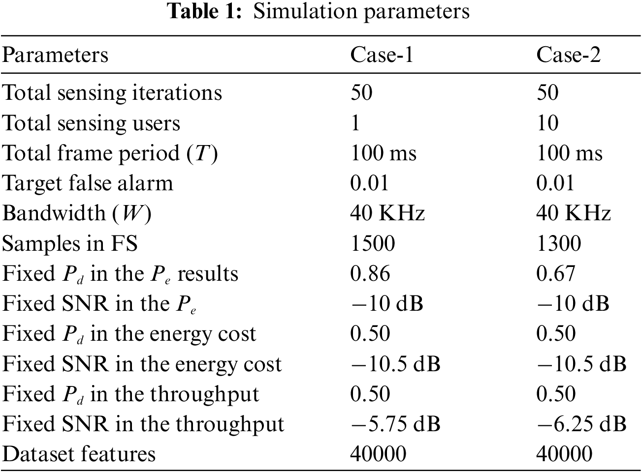
For the simulation setup, the SNRs vary from −15 to −10.25 dB in the presence of ten cooperative SUs. For 20 levels of detection probability ranging between 0.01 to 0.99, the false alarm probabilities in the dataset are ten. The corresponding number of samples is measured for each combination of these values. Hence, we get 40,000 samples in the dataset. The model is trained using SNRs, false alarms, and detection probability as the input features and samples as the output feature. The frame duration (T) is 100 ms, SNRs are fixed at −10.5 dB when the detection probability varies. For the FS scheme, the total number of samples is 1500 and 1300 in case 1 and case 2. The false alarm probability is fixed in the test phase, while the detection probability varies from 0.50 to 0.99 to get the throughput, energy cost, and error probabilities. Similarly, the channel bandwidth and sampling frequency are kept as 40 KHz.

The simulation environment splits into two scenarios shown as case 1 and case 2 in Tab. 1. Throughput, sensing cost, and error probabilities are investigated in case 1 for the non-cooperative environment to sense the PU channel using the single-user fixed sample (SFS), single-user decision tree (SDT), single-user linear regression (SLR), and single-user FKNN (SFKNN). On the other hand, case 2 compares the proposed FKNN algorithm-based CSS with the DT and traditional FS schemes when all SUs participate in sensing and reporting PU channel data to the FC.

4.1 Case 1: Single User Sensing

Case 1 addresses the throughput, energy cost, and error probabilities at different levels of the SNRs and detection probabilities for the SFS and compared with the reconfigured sample estimation of the SFKNN, SDT, and SLR in Figs. 5–10. Fig. 5 exhibits the throughput performance achieved with the SFKNN, SFS, SDT, and SLR schemes. These results confirm that the SFS achieves low channel throughput confronted with the SFKNN, SLR, and SDT at different levels of the SNRs. Also, the results reveal that an increase in the SU SNRs leads to an increase in throughput performance. Likewise, the throughput performance of the SFKNN, SLR, SDT, and SFS in the case of a single user is shown in Fig. 6 at different levels of the detection probabilities. The result in Fig. 6 shows a dominant performance of the SFKNN scheme compared with SFS, SDT, and SLR. The proposed SFKNN results in Figs. 5 and 6 are next followed by the SDT scheme, while the SFS gets the minimum throughput results.

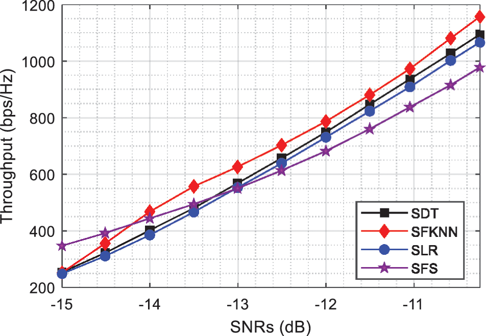
Figure 5: Throughput vs. SNRs (dB)

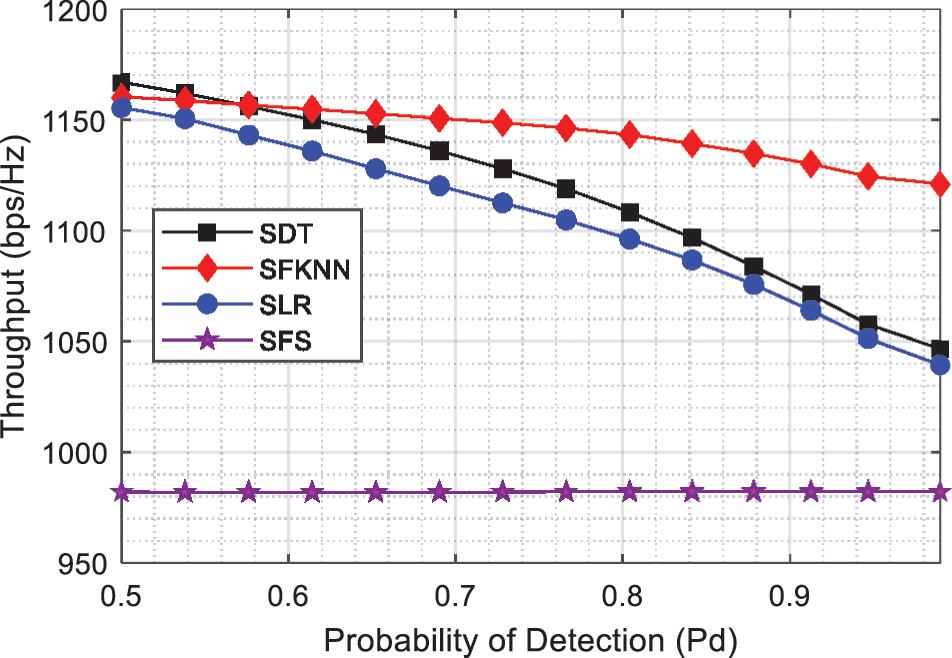
Figure 6: Throughput vs. probability of detection (Pd)

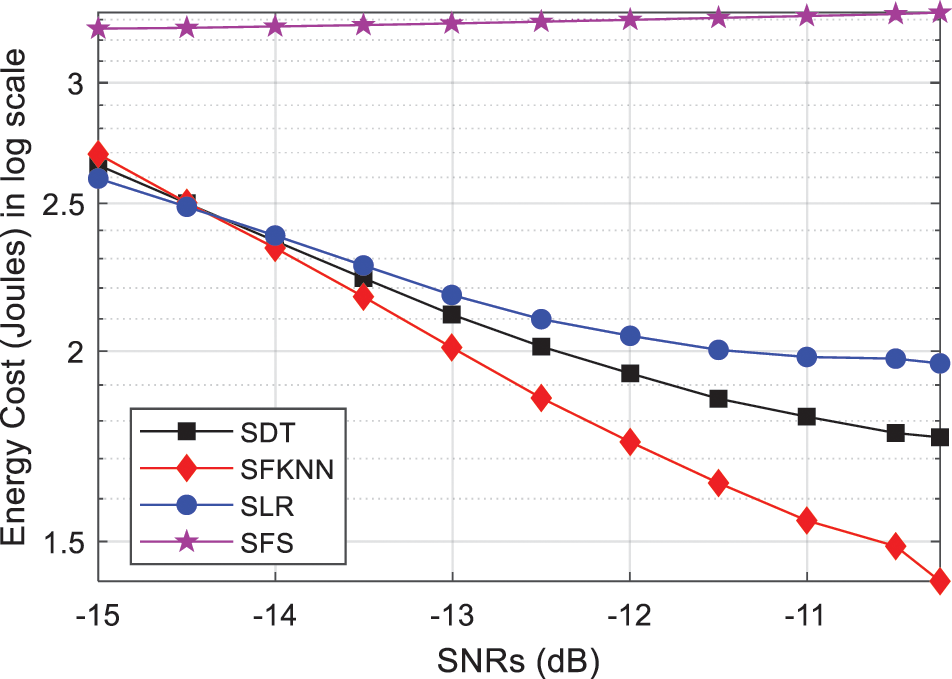
Figure 7: Energy cost vs. SNRs (dB)

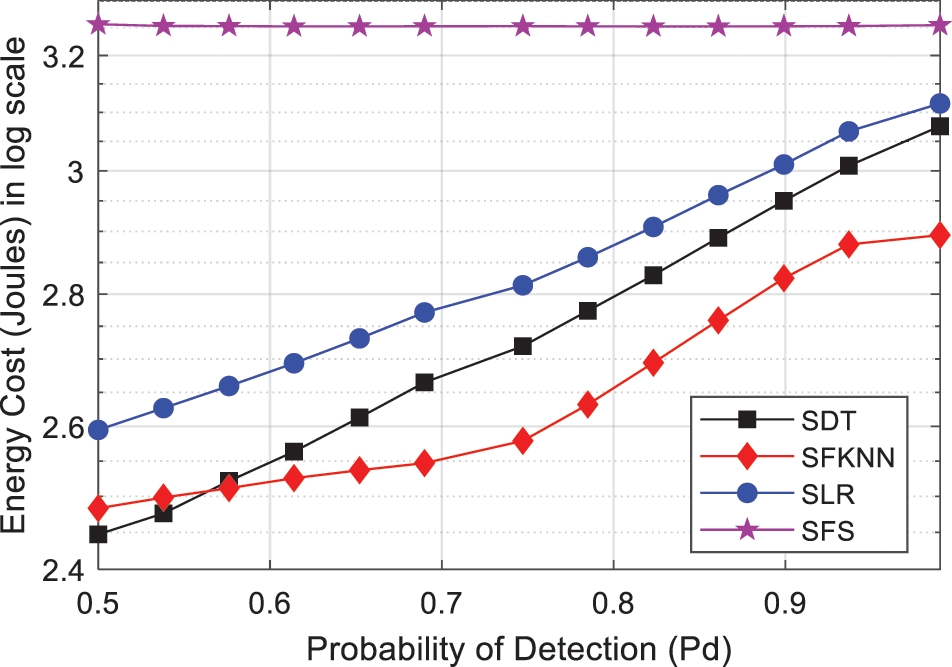
Figure 8: Energy cost vs. Probability of detection (Pd)

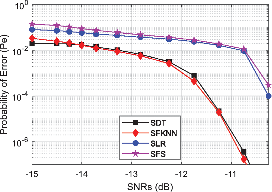
Figure 9: Probability of error (Pe) vs. SNRs (dB)

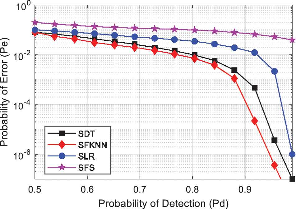
Figure 10: Probability of error (Pe) vs. Probability of detection (Pd)

The energy cost relation for the SFKNN, SDT, SLR, and SFS schemes at different levels of the SNRs and detection probability are shown in Figs. 7 and 8. Fig. 7 shows that SFS consumes more sensing energy with a high sensing cost for the SFS as compared with the SFKNN, SDT, and SLR. Similarly, the energy cost function of the SFS, SFKNN, SLR, and SDT in Fig. 8 against the increasing requirement of target detection probabilities proves high energy cost for the SFS compared with the SFKNN, SDT, and SLR.

The energy cost relation in Figs. 7 and 8 show the SNR and detection probability demands to measure the system energy cost. In Fig. 7 energy cost of the system decreases with increasing SNRs demand of the SUs, while in case of the high demand of the PU detection probability the system energy cost increases. To achieve high detection probability, more time is consumed by the SUs in sensing resulting in the high energy cost of the system.

Finally, the error probability results in sensing the PU channel while employing SFS, SFKNN, SDT, and SLR schemes are shown in Figs. 9 and 10. The error probability results in Fig. 9 infer the dominant performance of the SFKNN as compared with SDT, SLR, and SFS-based individual user sensing. An increase in the value of the SNRs and fixed detection probability in Fig. 9 lowers the SFKNN error probability related to the SLR, SFS, and SDT based schemes. Fig. 10 depicts the error probability results for the SFKNN, SLR, SDT, and SFS under fixed SNRs and changing detection probability. Fig. 10 shows that SFKNN has minimum sensing error followed by the SDT and SLR schemes, while the SFS performance is poor due to high sensing error. It is observable that increasing demand for high detection probability and SNRs at the SU leads to reduce error probability of the system.

It is concluded from the results in case 1 that SFKNN has the best sensing performance when individual SU sense the PU activity. The SFKNN effectively finds the optimum number of sensing samples to achieve high throughput, minimum energy cost, and low sensing error. An increase in the sensing time for the FS produces better sensing accuracy with the cost of more sensing energy and reduces the channel throughput.

4.2 Case 2: Cooperative Sensing

Case 2 illustrates the error probabilities in the FC decision while employing EGC, MGC, and count combination schemes for global decisions. Here ML techniques such as FKNN and FS-based DT are used to find the optimal sensing samples that further lead to minimum sensing error with lower energy cost and high average throughput. It can be seen from the result in case 2 that the proposed FKNN based combination has improved average throughput with low energy cost and minimum error in sensing the PU channel.

Fig. 11 shows the average throughput of the cooperative SUs against raising SNRs with target detection probability for the FKNN, DT, and FS schemes. This shows a high average throughput accomplishment of the FKNN compared with the DT and FS when target SNRs for the cooperative SUs increases. The proposed scheme is followed by the DT algorithm, while the FS has a low average throughput. Fig. 12 shows the average throughput performance for the proposed FKNN, DT, and FS-based schemes at different levels of the target detection probabilities under fixed SNRs. The results in the figure show that for the demand of improved detection probability of the SUs severe decrease in the average throughput of the DT and FS-based combination schemes is observed. The simple FS scheme has the least average throughput performance at all values of the target detection probabilities.

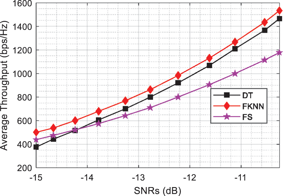
Figure 11: Average throughput vs. SNRs (dB)

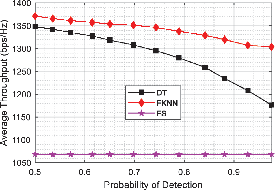
Figure 12: Average throughput vs. probability of detection (dB)

Figs. 13 and 14 show the comparison of the energy cost of the CSS for the proposed FKNN algorithm, DT, and FS against varying SNRs and target detection probabilities. It is visible from the results in Fig. 13 that the FKNN estimated sensing samples have low energy costs in CSS as compared with the DT and FS for increasing demand of SNRs and fixed detection probabilities. The FKNN results are followed by the DT, while the FS shows a higher energy cost. Fig. 13 shows the high energy cost in CSS by the DT scheme compared with the FS scheme when the SNRs are below −13 dB. The DT scheme in these results dominates the FS scheme as the SNR is allowed to pass −13 dB.

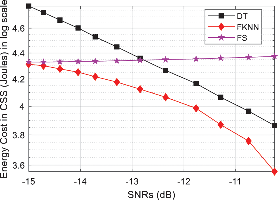
Figure 13: Energy cost vs. SNRs (dB)

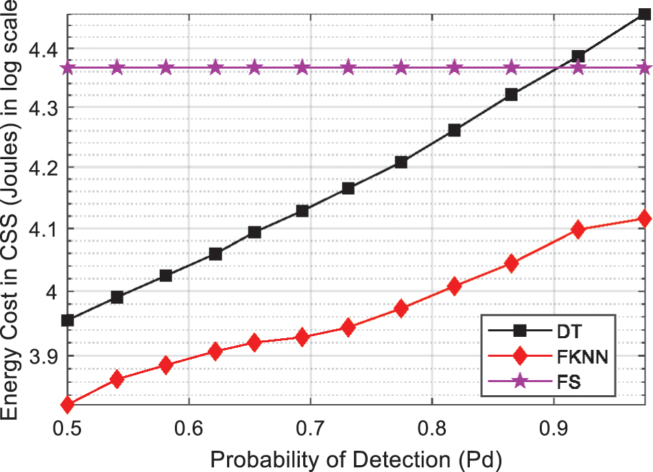
Figure 14: Energy cost vs. probability of detection (Pd)

Fig. 14 address the energy cost in CSS against the increasing demand of detection probabilities and fixed SNRs. The result shows that the proposed FKNN algorithm has the minimum energy cost at various detection probabilities. The DT scheme in Fig. 14 shows that to meet the demands of high detection probability for the DT-based CSS, the energy cost increase more compared with the FKNN.

The FKNN is less affected in energy cost for the increasing demands of detection probabilities and SNRs compared with the DT and FS technique.

It can be seen from the results given in Figs. 11–14 that the FKNN based CSS attains high average throughput with minimum energy cost as compared with the DT and FS schemes. To exhibit the cost paid by the proposed scheme in terms of error probabilities, simulation results are illustrated in Figs. 15 and 16. These results are achieved for the MGC, EGC, and count decision schemes, while employing FKNN estimated samples, DT estimated samples and FS techniques. Fig. 15 shows that FKNN based MGC, EGC, and count decisions have the minimum sensing error at all values of the SNRs when the target detection probability is fixed. The MGC with FKNN (MGC-FKNN), EGC with FKNN(EGC-FKNN), and Count with FKNN (Count-FKNN) results are followed by the DT algorithm based on MGC with DT (MGC-DT), EGC with DT (EGC-DT), and Count with DT (Count-DT). The MGC with FS (MGC-FS), EGC with FS (EGC-FS), and Count with FS (Count-FS) are shown to have high sensing errors in detecting PU channels. Similarly, Fig. 16 shows the error probability results against the varying target detection probabilities and fixed SNRs. The EGC-FKNN produces improved detection with minimum sensing error at different levels of the target detection probabilities. The Count-FS, EGC-FS, and MGC-FS schemes have their worst sensing performance with high sensing error in the global decisions. It can be concluded from the results in case 2 that the employment of FKNN for sensing PU channel achieves higher average throughput, low energy cost, and minimum sensing error for the EGC, MGC, and Count decision schemes.

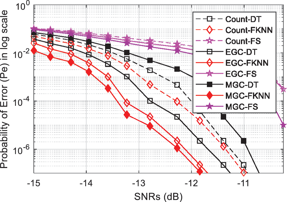
Figure 15: Probability of error (Pe) vs. SNRs (dB)

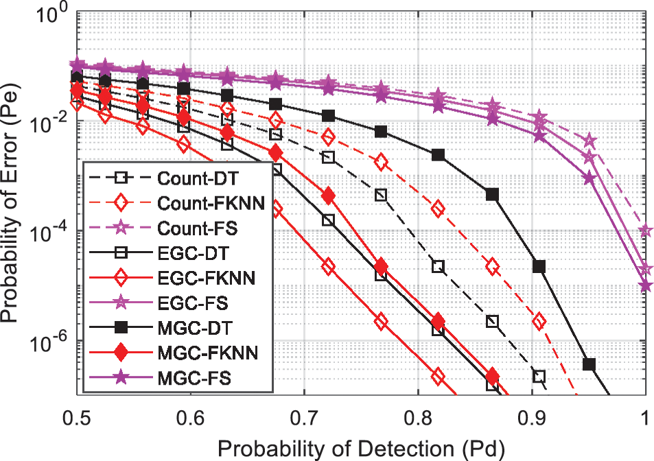
Figure 16: Probability of error (Pe) vs. probability of detection (Pd)

5  Conclusion

Spectrum sensing is the most significant task in CRN to access the PUs spectrum and minimize the disturbances for legitimate users. CSS is one way to accomplish reliable sensing results in the Raleigh fading environment. SUs are essentially required to decide instantly with minimum sensing time, ensuring decision reliability. In the non-reconfigurable sensing time, low sensing samples increase the channel throughput and reduce energy consumption with the cost of a decrease in sensing reliability. However, with the increased in sensing time, sensing accuracy enhances at the cost of reduced channel throughput and increased energy consumption. Therefore, this paper proposed an FKNN-based ML scheme to find the optimal sensing time resulting in higher throughput and reduced energy consumption with better sensing reliability. The effectiveness of the proposed scheme is validated by comparing the results with the traditional FS, LR, and DT schemes.

Funding Statement: This work was supported in part by the Ministry of Science and ICT (MSIT), Korea, under the Information and Technology Research Center (ITRC) support program (IITP-2022-2018-0-01426) and in part by the National Research Foundation of Korea (NRF) funded by the Korea government (MSIT) (No. 2021R1A2C1013150).

Conflicts of Interest: The authors declare that they have no conflicts of interest to report regarding the present study.

References

 1.  J. Mitola and G. Q. Maguire, “Cognitive radio: Making software radios more personal,” IEEE Personal Communications, vol. 6, no. 4, pp. 13–18, 1999. [Google Scholar]

 2.  S. Haykin, “Cognitive radio: Brain-empowered wireless communications,” IEEE Journal on Selected Areas in Communications, vol. 23, no. 2, pp. 201–220, 2005. [Google Scholar]

 3.  Q. Wu, G. Ding, Y. Xu, S. Feng, Z. Du et al., “Cognitive internet of things: A new paradigm beyond connection,” IEEE Internet of Things Journal, vol. 1, no. 2, pp. 129–143, 2014. [Google Scholar]

 4.  Y. Arjoune and N. Kaabouch, “A comprehensive survey on spectrum sensing in cognitive radio networks: Recent advances, new challenges, and future research directions,” Sensors (Switzerland), vol. 19, no. 1, pp. 1–32, 2019. [Google Scholar]

 5.  A. Ranjan, Anurag and B. Singh, “Design and analysis of spectrum sensing in cognitive radio based on energy detection,” in 2016 Int. Conf. on Signal and Information Processing IConSIP 2016, Nanded, India, pp. 1–5, 2017. [Google Scholar]

 6.  I. Ilyas, S. Paul, A. Rahman and R. K. Kundu, “Comparative evaluation of cyclostationary detection based cognitive spectrum sensing,” in 2016 IEEE 7th IEEE Annual Ubiquitous Computing, Electronics and Mobile Communication Conf., New York, NY, USA, pp. 2–8, 2016. [Google Scholar]

 7.  I. F. Akyildiz, B. F. Lo and R. Balakrishnan, “Cooperative spectrum sensing in cognitive radio networks: A survey,” Physical Communication, vol. 4, no. 1, pp. 40–62, 2011. [Google Scholar]

 8.  D. Cabric, S. M. Mishra and R. W. Brodersen, “Implementation issues in spectrum sensing for cognitive radios,” in Signals, Systems and Computers, 2004 Conf. Record of the Thirty-Eighth Asilomar Conf. on, Pacific Grove, CA, USA, pp. 772–776, 2004. [Google Scholar]

 9.  N. Gul, M. S. Khan, J. Kim and S. M. Kim, “Robust spectrum sensing via double-sided neighbor distance based on genetic algorithm in cognitive radio networks,” Mobile Information Systems, vol. 2020, no. 1, pp. 1–10, 2020. [Google Scholar]

10. D. Lee, “Adaptive random access for cooperative spectrum sensing in cognitive radio networks,” Wireless Personal Communications, vol. 14, no. 2, pp. 831–840, 2015. [Google Scholar]

11. Y. He, J. Xue, T. Ratnarajah, M. Sellathurai and F. Khan, “On the performance of cooperative spectrum sensing in random cognitive radio networks,” IEEE Systems Journal, vol. 12, no. 1, pp. 881–892, 2018. [Google Scholar]

12. N. Gul, I. M. Qureshi, A. Elahi and I. Rasool, “Defense against malicious users in cooperative spectrum sensing using genetic algorithm,” International Journal of Antennas and Propagation, vol. 2018, pp. 1–11, 2018. [Google Scholar]

13. D. Hamza, S. Aïssa and G. Aniba, “Equal gain combining for cooperative spectrum sensing in cognitive radio networks,” IEEE Transactions on Wireless Communication, vol. 13, no. 2, pp. 4334–4345, 2014. [Google Scholar]

14. R. Biswas, J. Wu and X. Du, “Mitigation of the spectrum sensing data falsifying attack in cognitive radio networks,” Cyber-Physical Systems, vol. 7, no. 3, pp. 159–178, 2021. [Google Scholar]

15. N. Gul, I. M. Qureshi, A. Omar, A. Elahi and S. Khan, “History-based forward and feedback mechanism in cooperative spectrum sensing including malicious users in cognitive radio network,” PLoS One, vol. 12, no. 8, pp. e0183387, 2017. [Google Scholar]

16. N. Gul, I. M. Qureshi, S. Akbar, M. Kamran and I. Rasool, “One-to-many relationship based kullback leibler divergence against malicious users in cooperative spectrum sensing,” Wireless Communications and Mobile Computing, vol. 2018, no. 1, pp. 1–14, 2018. [Google Scholar]

17. M. Jenani, “Network security, a challenge,” International Journal of Advanced Networking and Applications, vol. 8, pp. 120–123, 2017. [Google Scholar]

18. N. Gul, I. M. Qureshi, M. S. Khan, A. Elahi and S. Akbar, “Differential evolution based reliable cooperative spectrum sensing in the presence of malicious users,” Wireless Personal Communications, vol. 114, no. 2, pp. 123–147, 2020. [Google Scholar]

19. I. S. Trubin, “Security threats in mobile cognitive radio networks,” in Proc. 2018 IEEE East-West Design and Test Symp., EWDTS 2018, Kazan, Russia, pp. 1–6, 2018. [Google Scholar]

20. N. Gul, I. M. Qureshi, A. Naveed, A. Elahi and I. Rasool, “Secured soft combination schemes against malicious-users in cooperative spectrum sensing,” Wireless Personal Communications, vol. 108, no. 4, pp. 389–408, 2019. [Google Scholar]

21. N. Gul, M. S. Khan, S. M. Kim, J. Kim and I. Ullah, “Particle swarm optimization in the presence of malicious users in cognitive IoT networks with data,” Scientific Programming, vol. 2020, no. 2, pp. 1–11, 2020. [Google Scholar]

22. Y. C. Liang, Y. Zeng, C. Y. Edward and A. T. Hoang, “Sensing-throughput tradeoff for cognitive radio networks,” IEEE Transaction on Wireless Communication, vol. 7, no. 4, pp. 1–12, 2008. [Google Scholar]

23. A. El-Mougy, M. Ibnkahla, G. Hattab and W. Ejaz, “Reconfigurable wireless networks,” Proceedings of the IEEE, vol. 103, no. 7, pp. 1125–1158, 2015. [Google Scholar]

24. P. Paysarvi-Hoseini and N. C. Beaulieu, “Optimal wideband spectrum sensing framework for cognitive radio systems,” IEEE Transactions on Signal Processing, vol. 59, no. 3, pp. 1170–1182, 2011. [Google Scholar]

25. P. Paysarvi-Hoseini and N. C. Beaulieu, “On the benefits of multichannel/wideband spectrum sensing with non-uniform channel sensing durations for cognitive radio networks,” IEEE Transactions on Communications, vol. 60, no. 9, pp. 2434–2443, 2012. [Google Scholar]

26. Y. Pei, Y. C. Liang, K. C. Teh and K. H. Li, “Sensing-throughput tradeoff for cognitive radio networks: A multiple-channel scenario,” in IEEE Int. Symp. on Personal, Indoor and Mobile Radio Communications, PIMRC, Tokyo, Japan, pp. 1257–1261, 2009. [Google Scholar]

27. N. Abbas, Y. Nasser and K. E. Ahmad, “Recent advances on artificial intelligence and learning techniques in cognitive radio networks,” Eurasip Journal on Wireless Communications and Networking, vol. 2015, no. 1, pp. 1–20, 2015. [Google Scholar]

28. Z. Qin, X. Zhou, L. Zhang, Y. Gao, Y. C. Liang et al., “20 years of evolution from cognitive to intelligent communications,” IEEE Transactions on Cognitive Communications and Networking, vol. 6, no. 1, pp. 6–20, 2020. [Google Scholar]

29. A. Balieiro, P. Yoshioka, K. Dias, C. Cordeiro and D. Cavalcanti, “Adaptive spectrum sensing for cognitive radio based on multi-objective genetic optimization,” Electronics Letters, vol. 49, no. 17, pp. 1099–1101, 2013. [Google Scholar]

30. A. Toma, A. Krayani, M. Farrukh, Q. Haoran, L. Marcenaro et al., “AI-based abnormality detection at the phy-layer of cognitive radio by learning generative models,” IEEE Transactions on Cognitive Communications and Networking, vol. 6, no. 1, pp. 21–34, 2020. [Google Scholar]

31. K. A. Yau, P. Komisarczuk and P. D. Teal, “Applications of reinforcement learning to cognitive radio networks,” in 2010 IEEE Int Conf. Commun Work ICC 2010, Cape Town, South Africa, pp. 1–6, 2010. [Google Scholar]

32. Y. Wang, X. Tang, G. J. Mendis, J. Wei-Kocsis, A. Madanayake et al., “AI-driven self-optimizing receivers for cognitive radio networks,” in 2019 IEEE Cognitive Communications for Aerospace Applications Workshop, CCAAW 2019, Cleveland, OH, USA, pp. 1–4, 2019. [Google Scholar]

33. L. Yu, Y. Guo, Q. Wang, C. Luo, M. Li et al., “Spectrum availability prediction for cognitive radio communications: A dcg approach,” IEEE Transactions on Cognitive Communications and Networking, vol. 6, no. 2, pp. 476–485, 2020. [Google Scholar]

34. S. Zheng, S. Chen, P. Qi, H. Zhou and X. Yang, “Spectrum sensing based on deep learning classification for cognitive radios,” China Communications, vol. 17, no. 2, pp. 138–148, 2020. [Google Scholar]

35. P. Zu, J. Li, D. Wang and X. You, “Machine-learning-based opportunistic spectrum access in cognitive radio networks,” IEEE Wireless Communications, vol. 27, no. 1, pp. 38–44, 2020. [Google Scholar]

36. S. Liu, I. Ahmad, Y. Bai, Z. Feng, Q. Zhang et al., “A novel cooperative sensing based on spatial distance and reliability clustering scheme in cognitive radio system,” in IEEE Vehicular Technology Conf., Las Vegas, NV, USA, pp. 1–5, 2013. [Google Scholar]

37. Z. Javed, K. A. Yau, H. Mohamad, N. Ramli, J. Qadir et al., “RL-budget: A learning-based cluster size adjustment scheme for cognitive radio networks,” IEEE Access, vol. 6, pp. 1055–1072, 2017. [Google Scholar]