A Productivity Prediction Method Based on Artificial Neural Networks and Particle Swarm Optimization for Shale-Gas Horizontal Wells

1  Introduction

Predrilling prediction of productivity for shale gas horizontal wells is an important link in the formulation and optimization of development schemes for shale gas. It provides an assessment basis for the investment risk of shale reservoir development and is particularly important for guiding the development [1–4].

However, the current productivity prediction technology for shale gas horizontal wells is not yet mature. These technologies mainly include physical simulation methods, empirical formula methods, analytical methods and numerical simulation. Notably, analytical methods can only study the two-dimensional seepage process of single-phase fluids in homogeneous formations, it can not predict the production of gas wells with complex gas deposits [5–8]. The physical simulation method mainly includes electrical simulation and the use of sand pack models for research. However, the electricity analogy experiment is not suitable for evaluating production under a complex and unsteady state [9]. Although the sand packs model is suitable for studying fluid seepage mechanism under formation temperature and pressure, it is difficult to simulate the initiation and propagation of fractures and the stress sensitivity of the reservoir. In addition, it requires the establishment of a three-dimensional reservoir physical model to ensure its accuracy. Thus, the method is not applicable by the fact that the model is complex, the experiment is difficult, and it takes a long time [10]. The above limitations suggest that it is difficult to obtain accurate regression equations for models based on empirical formula methods. Moreover, the equations are usually for individual shale gas horizontal wells or individual blocks, and thus the generalization ability of this method is relatively poor [11]. On the other hand, numerical simulation methods for predicting productivity also have many problems: (1) Physical parameters of the reservoir are changeable and multi-scale problems are prominent, which makes it difficult to establish a reasonable geological model. (2) There is a large demand for evaluation parameters, but they are difficult to obtain before drilling. (3) Researchers usually devote their work to the study of seepage mechanism in shale matrix or fractures, without considering the characteristics of fracture networks [12–16]. (4) Shale has poor physical characteristics and strong stress sensitivity. To sum up, shale gas development is affected by many uncertain factors, which makes the current deterministic productivity prediction methods poor in reliability [17,18]. Considering the uncertainty of shale gas development, non-deterministic prediction methods of shale gas productivity is an effective way to solve the above-mentioned problems. However, the existing non-deterministic prediction methods are only applicable to shale gas wells after they are put into production [19,20].

ANN is a new artificial intelligence method developed on biological research. It has the ability to learn and solve complex nonlinear problems through self-learning. Currently, machine-learning methods have been widely applied to estimate oil and coalbed methane well production performance [21–23]. There are only few reports in the literature on predicting the productivity of shale gas wells based on the machine learning methods, which also as comprehensively as possible considers the combined influence of geological and engineering parameters, because shale gas development is affected by many uncertain factors as mentioned above.

No matter what problems the machine learning methods have solved, an enlarged database is an important prerequisite to obtain a satisfactory prediction performance and improve the generalisation capability of the model [24–26]. This study collected 317 data samples obtained from the production data of 317 horizontal shale gas wells in the Sichuan Basin including nine wells in Luzhou Block, 10 wells in Yuxi Block, 233 wells in Changning Block, 58 wells in Weiyuan Block, and seven wells in Zigong Block. Every data sample included eight geological parameters (pressure coefficient, vertical depth, TOC, porosity, Young’s modulus, total gas content, Poisson’s ratio, and brittleness index) and seven engineering parameters (displacement, cluster number, fluid intensity, flow back rate, slick water ratio, sanding intensity, and quartz sand ratio). On the basis of the cross-regional and invaluable dataset, this study constructed three new artificial intelligence methods for predicting the productivity of shale gas horizontal wells on the basis of the ANN combined with PSO, ICA and ACO. They were abbreviated as PSO-ANN, ICA-ANN, and ACO-ANN models. The methods starting from actual data, and accurately predicting shale gas production are of great significance for determining the rational development decision of shale gas wells [27,28].

2  Specification of the Study

2.1 Artificial Neural Network

The artificial neural network is composed of a large number of neurons interconnected. The function of each neuron is relatively simple that performs the following commands:

Y=max(0,∑iwiXi+a) (1)

where Y is the neuron output; wi are the weights; Xi are the neuron inputs and a is bias.

All neurons which are set in different layers are connected by weights, and the function between inputs and outputs is conducted as follows:

Hi=max(0,wi⋅Hi−1+ai),1≤i≤K,H0=X (2)

Y=max(0,V⋅HK) (3)

where matrices wi, V and vector ai are model parameters; L is the number of layers.

The network is trained by performing optimization of weights until the output values are as close as possible to the actual outputs. The architecture of the ANN was turned based on the mean squared error (MSE), which is defined as:

MSE=1M∑i=1M(Yi∗−Yi)2 (4)

where M is the number of data samples; Yi* and Yi are the predicted and true values of the test production per unit well length.

2.2 Particle Swarm Optimization (PSO)

PSO can find the optimum through information sharing between individuals in the swarm [29]. The PSO is a group of random swarm of particles (random solution) and each represented a specific ANN architecture, then PSO can find the optimum iteratively. In each iteration, the particle updates its position and velocity by comparing the fitness of each particle and the two extremum (one is the individual extremum of the particle and the other is the global extremum of entire swarm). The particle approaches the best position in its own history until the end of iterations. The fitness of particles was evaluated by the MSE on the training set.

The particles update the position formula by the following formula:

VjL+1m=ωLVjLm+a1f1(KjLm−XiLm)+a2f2(ULm−XjLm) (5)

j=1,2⋯L=1,2⋯

XjL+1m=XjLm+VjL+1m (6)

where a real vector is used to represent the position of a single particle. XjLm and XjL+1m represent the positions of particle j at iteration L and L + 1 in the mth dimension. VjLm and VjL+1m represent the velocity of the particle j at iteration L and L + 1 in the mth dimension. KjLm and GjLm represent the best position of a particle and the swarm best position. a1 and a2 are the inertia parameter. f1 and f2 are random numbers between 0 and 1.

ω(k)=ωmax−k(ωmax−ωmin)Tmax (7)

where the k is the current iteration number of swarm; Tmax is the maximum iteration number set; ωmax is the maximum inertia weight, and ωmin is the minimum inertia weight. ωmax is generally set to be 0.9, and ωmin is generally set to be 0.4.

The flowchart of the PSO algorithm is demonstrated in Fig. 1.

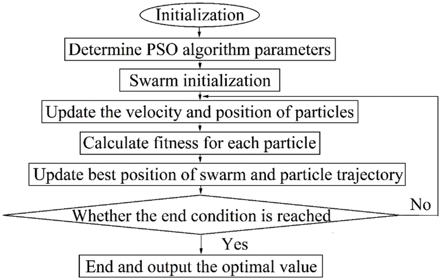
Figure 1: Flowchart of the PSO algorithm

2.3 Imperialist Competitive Algorithm (ICA)

ICA starts with initial populations called countries [30]. There are two types of countries: colony and imperialist. Attempting of the imperialists to gain more colonies was named imperialist competitive process. During the competition, the powerful imperialists will be more power and the weaker imperialists will be weaker. If an empire missed all of its colonies, the empire will be collapsed. In the end, the most powerful imperialist will remain in the world and all the countries are its colonies. Power and position of the imperialist and colonies at this level of computation are the same [31]. Fig. 2 shows the flow chart of ICA-ANN prediction model.

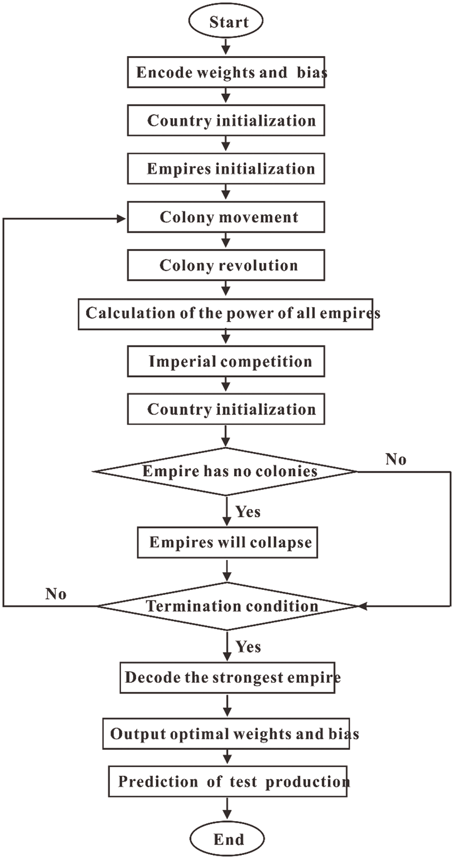
Figure 2: Flowchart of the ICA algorithm

2.4 Ant Clony Optimization (ACO)

ACO is a bionic intelligent optimization algorithm. Ant colony algorithm is inspired by the process of ants foraging, ants leave pheromones on their way to find food sources, and ants in the colony can sense pheromones and move along places with high pheromone concentrations, forming a positive feedback mechanism. After a period of time, the ants can determine an optimal path to the food source. The basic idea of optimizing ANN with ACO is: First, the elements of the weight matrix and the bias vector are taken out to form the path coordinates of the ant population. Because the shorter the ant’s path to the food source, the higher the pheromone content on the path, so the mean square error (MSE) is used as the ant’s fitness value. The shortest path determined by the final ant population is used as the optimal initial weight and bias. Then the optimal weight and bias were assigned to the ANN for training and testing, and the error is compared with the prediction of the ANN before optimization. Fig. 3 shows the flow chart of ACO-ANN prediction model.

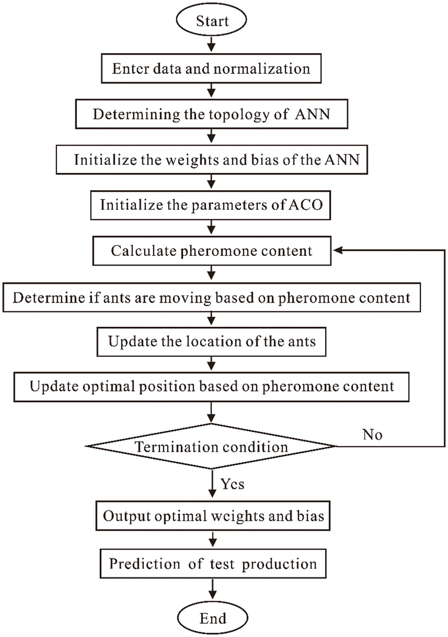
Figure 3: Flowchart of the ACO algorithm

2.5 Partial Dependency Graph (PDP)

PDP is a method used to determine the dependence of prediction on input variables. PDP represents the marginal impact of one or two features on the prediction results of the machine learning model, that is, how the variables affect the prediction results. The partial dependence function for regression is as follows:

f^xS(xS)=ExC[f^xS(xS,xC)]=∫f^xS(xS,xC)dP(xC) (8)

where xs represents the characteristic variable of interest and xc represents other variables.

A function f(xs) that only depends on xs can be obtained by integrating xc. This function is a partially dependent function because it can realize the interpretation of a single variable xs. In actual operation, the Monte Carlo method is used to determine the partial dependence function by calculating the average value of the training set. The specific formula is as follows:

f^xS(xS)=1n∑i=1nf^xS(xS,xC(i)) (9)

where n represents the sample size.

The specific implementation steps of the single variable PDP are as follows: (1) Select a characteristic variable of interest for research and define the searching grid. (2) Substitute each value in the searching grid into xs in the above PDP function, a black box model is used to make predictions and obtain average predicted values. (3) The relationship curve between the variable and the predicted value is the partial dependence graph.

3  Model Application

3.1 Dataset Collection and Characteristics

The shale gas horizontal well production is affected by geological factors and engineering factors. Geological parameters guide the comprehensive analysis of the target reservoir and effectively transform the target reservoir. Combining the previous production measures, production performance, and profile modification of adjacent wells can effectively improve the production of a single well through reasonable fracturing operation parameters.

Geological factors

When the vertical depth of shale reservoir increases, especially when it exceeds 3500 m, the horizontal in-situ stress difference of shale is large, the brittleness is weak, and the plasticity is strong, which is not conducive to the volume fracturing and fracture propagation of shale [32–34]. The pressure coefficient, TOC, total gas content, and porosity determine the quality of shale reservoir. High quality shale in the Sichuan Basin generally has high TOC, which is usually conducive to the development and preservation of shale pores [35–38]. The greater the Young’s modulus, the easier the fracture propagation and the more complex the fracture network. However, the fracture becomes narrow and the conductivity is weakened when Young’s modulus is too high [39–41]. The higher the Poisson’s ratio, the greater the formation fracture pressure and closure pressure, the smaller the fracture height, and the smaller the effective fracturing volume of shale reservoir [42]. Brittleness index reflects the content of brittle minerals in shale, and high brittleness index is conducive to volume fracturing and fracture propagation of shale [43–45].

Engineering factors

Studies have reported that reasonable distribution of cluster spacing is conducive to the increase of stimulated reservoir volume [46–48]. Displacement is the most effective factor for determining the net pressure, and the net pressure is the key to the formation of complex fracture network [49]. The flow-back rate is closely related to the spontaneous imbibition of fracturing fluid, which spontaneously imbibes into the reservoir because of the huge capillary pressure of the reservoir, thereby displacing more gas into the fractures near the well and increasing the initial productivity [50–51]. Reasonable flow-back rate is also conducive to the increase of stimulated reservoir volume. High liquid consuming intensity can also increase the transportation distance of proppant, and make proppant effectively enter the branch and bedding fractures, which is conducive to the effective support of fractures and maintenance of long-term conductivity [52]. Studies have revealed that increasing the proppant injection intensity is conducive to the effective support of the fracture and maintenance of long-term conductivity [53]. The slick water needs to be compounded with linear gel in order to form a variable viscosity slick water system and thus meet the requirements of proppant transportation on site [54,55]. The relative density of quartz sand proppant is low, and it is convenient for construction and transportation. Ceramsite has high strength, low broken rate, and long bearing time, which helps to maintain fracture conductivity for a long time. Therefore, reasonable proppant proportion distribution is conducive to the effective support of multi-stage fractures and the maintenance of long-term conductivity [56].

Therefore, the above eight geological parameters and seven engineering parameters were selected as the key research variables. Fig. 4 shows the distribution of the 15 variables.

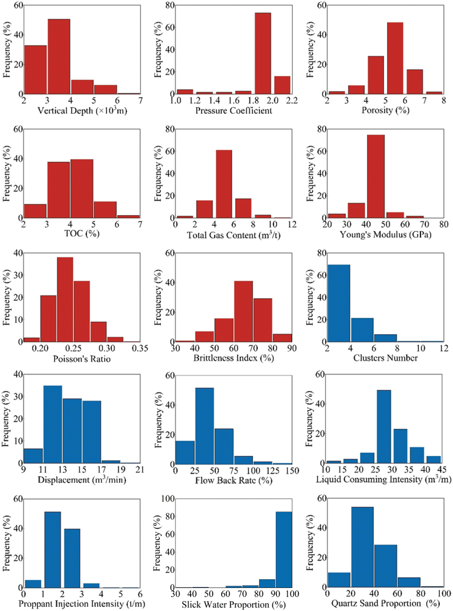
Figure 4: Distribution histogram of geological engineering parameters and test production

Fig. 5 shows the distribution of the test production per unit well length of the 317 shale gas wells. The dataset in this study was obtained from the production data of horizontal shale gas wells in the Sichuan Basin. In total, 317 data samples were collected, including nine wells in Luzhou Block, 10 wells in Yuxi Block, 233 wells in Changning Block, 58 wells in Weiyuan Block, and seven wells in Zigong Block, and the contingency and representativeness of the samples were avoided as much as possible. Moreover, the randomness and independence of the samples were strong to ensure the reliability of ANN model training.

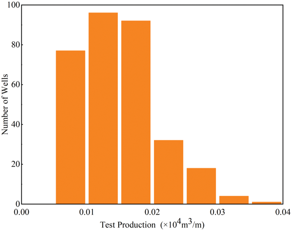
Figure 5: Distribution histogram of test production per unit well length

A normalized input signal can make the average of sample to be close to zero, which can accelerate the learning speed of the ANN model. In this study, the geological and engineering parameters of 317 shale gas wells were normalized as input variables of the ANN model according to Eq. (10). The normalized test productions per unit well length of the 317 shale gas wells were output variable of the ANN model in accordance with Eq. (11). The dataset was divided into the training set and testing set according to the ratio of nine to one. Ten-fold cross validation was used as the validation method.

Therefore, data samples including a shale gas horizontal well normalized test productions per unit well length, the eight geological parameters, and the seven engineering parameters were used in this study.

xi∗=xi−xminxmax−xmin (10)

yi∗=yi−yminymax−ymin (11)

where xi* represents normalized input variable; xi represents unnormalized input variable; xmin represents the minimum value of the input variable; xmax represents the maximum value of the input variable; yi* represents normalized output variables; yi represents unnormalized output variables; ymin represents the minimum value of the output variable; and ymax represents the maximum value of the output variable.

It is worth noting that the correlation between the input variables of the ANN model should not be too strong, otherwise, it will affect the accuracy of prediction. Fig. 6 shows the correlation coefficient (R) between the input variables. Results showed that the R between most variables was less than 0.5, indicating that there is a weak correlation between most input variables [57].

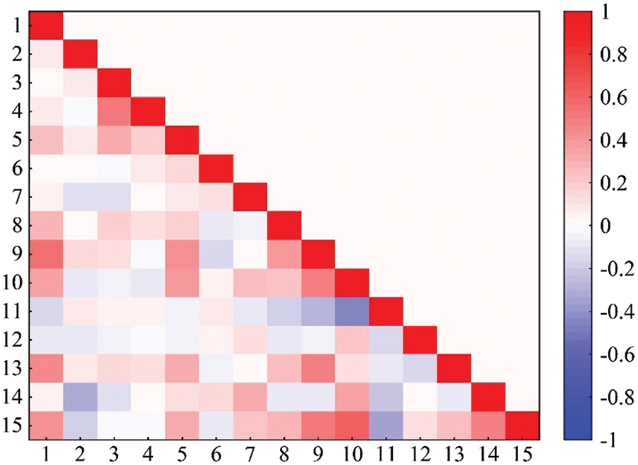
Figure 6: Input variable correlation heatmap

3.2 Structural Optimization

For the prediction of test productions per unit well length by the three artificial intelligence techniques, ANN model was developed first. Then, the PSO, ICA and ACO were used to optimize ANN model by optimizing the weights and biases. Simultaneously, based on trial tuning and experience, considering the complexity of input parameters, the tuning ranges for the number of neurons were 1-120. “trial and error” (TAE) was conducted with one and two hidden layers of ANN models. Ultimately, the ANN model 15-69-1 was defined as the best ANN technique for predicting test productions per unit well length in this study. The optimum ANN architecture used for further analysis is illustrated in Fig. 7.

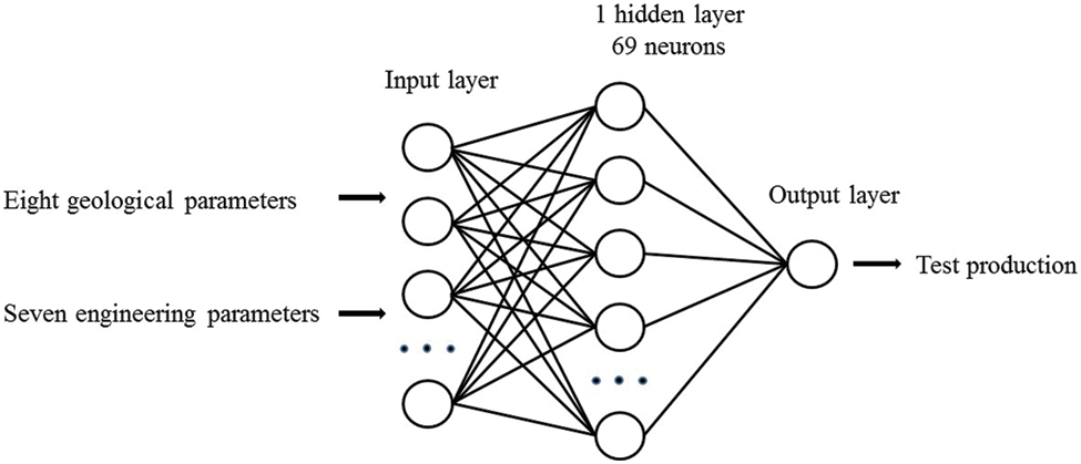
Figure 7: Optimum ANN architecture

3.3 Prediction of Test Productions Per Unit Well Length by the Meta-Heuristics Algorithms

3.3.1 PSO-ANN Model

The reliability of ANN model was evaluated by the statistical descriptors including coefficients of determination (R2)/Root-mean-square error (RMSE)/Slope of the regression line (k)/Willmott’s index of agreement (IA) were calculated between the predicted and actual shale gas test production per unit well length. Based on the statistical recommendation, a good prediction can be evaluated with R2 > 0.64, 0.85 < k < 1.15, or IA > 0.80 [58]. R2, RMSE, k and IA are defined as follows:

R2=1−∑i=1N(yi−yi∗)2∑i=1N(yi−y¯)2 (12)

RMSE=1N∑i=1N(yi−yi∗)2 (13)

k=∑yiyi∗∑(yi∗)2 (14)

IA=1−∑i=1N(yi−yi∗)2∑i=1N(|yi∗−y¯|+|yi−y¯|)2 (15)

where N represents the number of dataset; yi and yi* represent actual values and predicted values, respectively; y¯ and y¯ * represent the average predicted value and the average actual value, respectively.

The PSO algorithm parameters were set up before optimization of the ANN model as shown in Table 1.

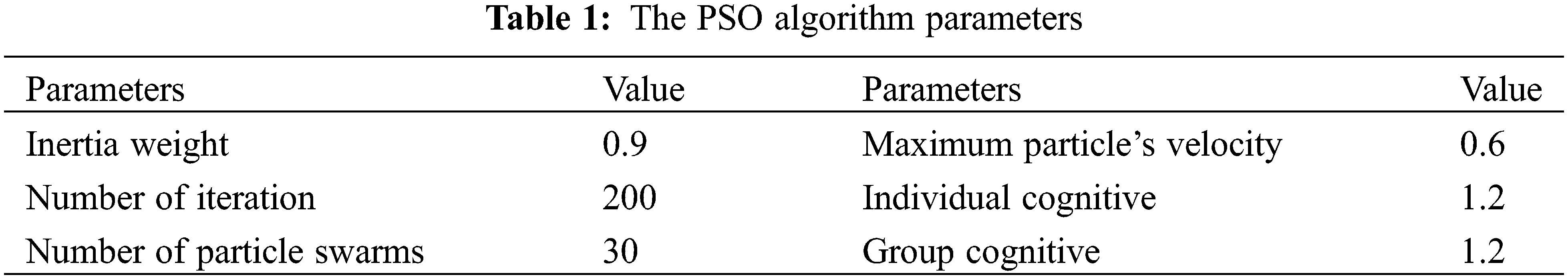
As shown in Fig. 8, a visible decrease in the swarm minimum RMSE was achieved as the number of iterations increased, indicating that PSO successfully optimized the ANN architecture. Figs. 9 and 10 showed that the PSO-ANN model successfully learned the relationships between the test production per unit well length and input variables. The predicting performance set of optimum ANN model on the training set is as follows: IA = 0.968, k = 0.986, RMSE = 0.0002, R2 = 0.876. The predicting performance set of optimum ANN model on the testing set is as follows: IA = 0.965, k = 0.957, RMSE = 0.0009, R2 = 0.847.

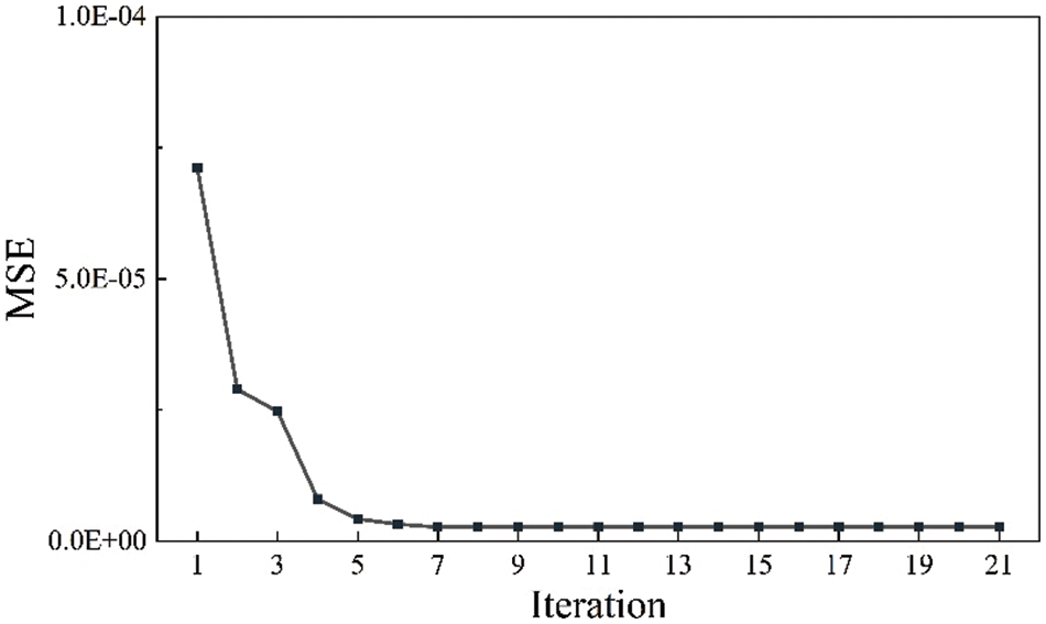
Figure 8: PSO-ANN performance in the training process

Figure 9: The predictive performance of PSO-ANN model on the training set

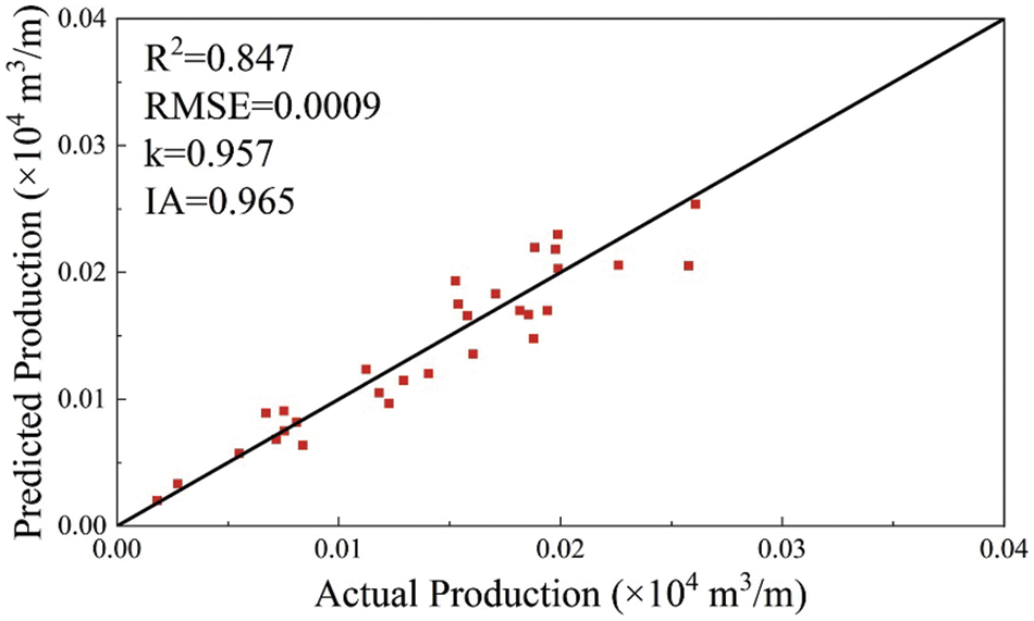
Figure 10: The predictive performance of PSO-ANN model on the testing set

3.3.2 ICA-ANN Model

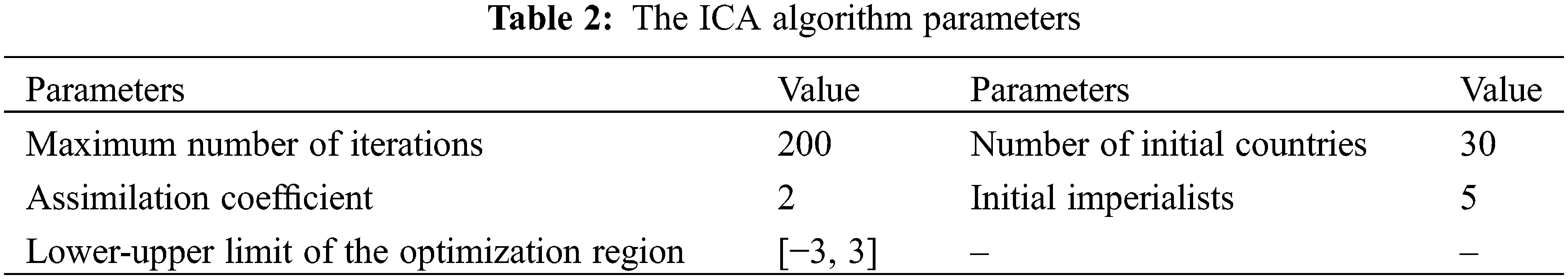
In this section, the ICA was used to optimize the weights and biases of the selected initialization ANN model. The ICA algorithm parameters were set up before optimization of the ANN model as shown in Table 2.

As shown in Fig. 11, a visible decrease in the swarm minimum RMSE was achieved as the number of iterations increased, indicating that ICA successfully optimized the ANN architecture. Figs. 12 and 13 showed that the ICA-ANN model successfully learned the relationships between the test production per unit well length and input variables. The predicting performance set of optimum ANN model on the training set is as follows: IA = 0.963, k = 0.986, RMSE = 0.0023, R2 = 0.867. The predicting performance set of optimum ANN model on the testing set is as follows: IA = 0.958, k = 0.946, RMSE = 0.0009, R2 = 0.842.

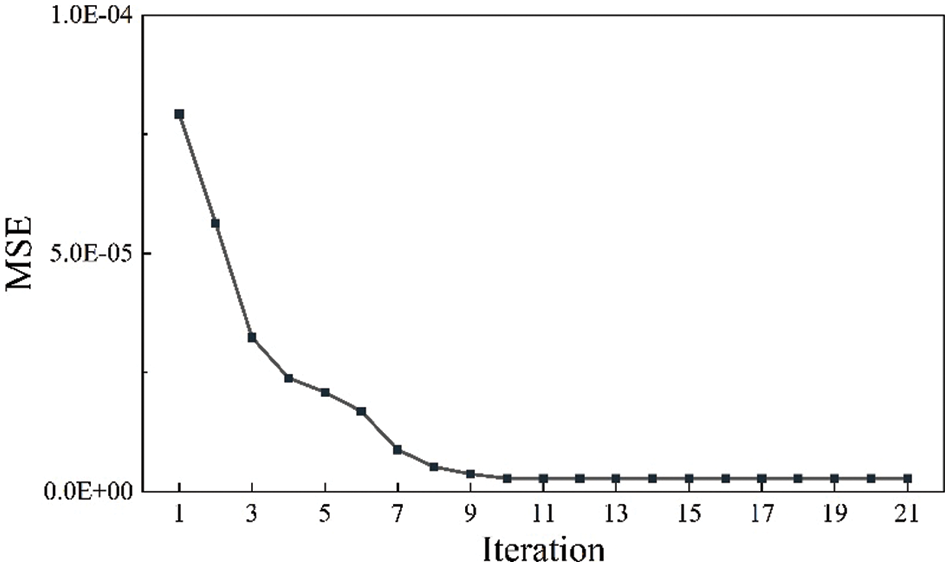
Figure 11: ICA-ANN performance in the training process

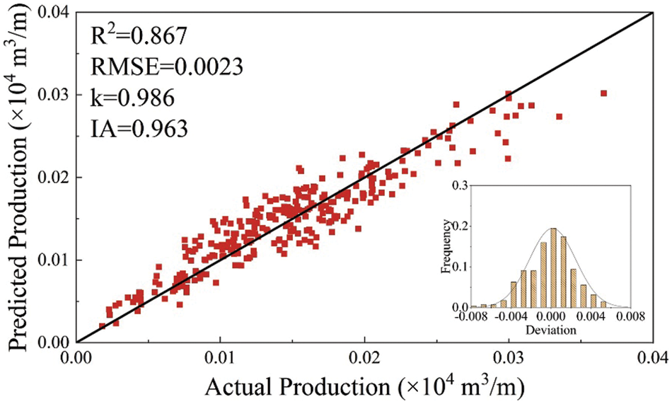
Figure 12: The predictive performance of ICA-ANN model on the training set

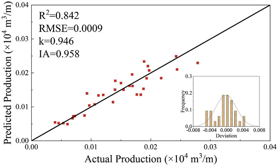
Figure 13: The predictive performance of ICA-ANN model on the testing set

3.3.3 ACO-ANN Model

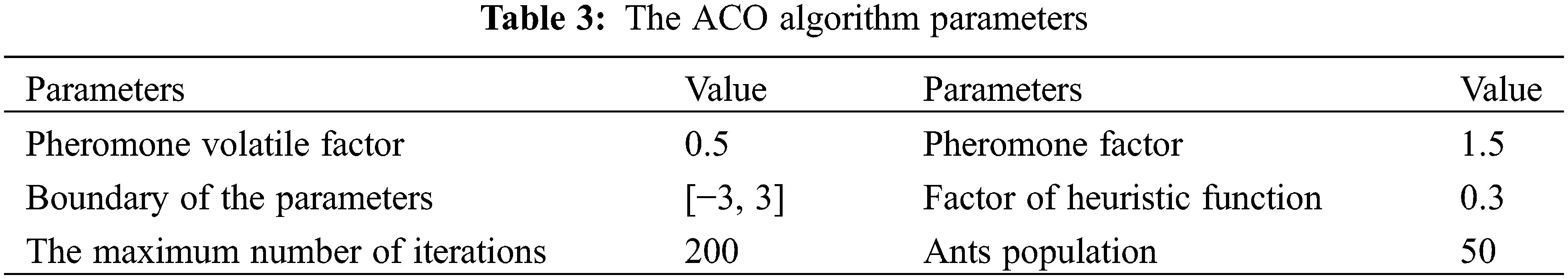
In this section, the ACO was used to optimize the weights and biases of the selected initialization ANN model. The ACO algorithm parameters were set up before optimization of the ANN model as shown in Table 3.

As shown in Fig. 14, a visible decrease in the swarm minimum RMSE was achieved as the number of iterations increased, indicating that ACO successfully optimized the ANN architecture. Figs. 15 and 16 showed that the ACO-ANN model successfully learned the relationships between the test production per unit well length and input variables. The predicting performance set of optimum ANN model on the training set is as follows: IA = 0.961, k = 0.966, RMSE = 0.0024, R2 = 0.862. The predicting performance set of optimum ANN model on the testing set is as follows: IA = 0.954, k = 0.951, RMSE = 0.0009, R2 = 0.838.

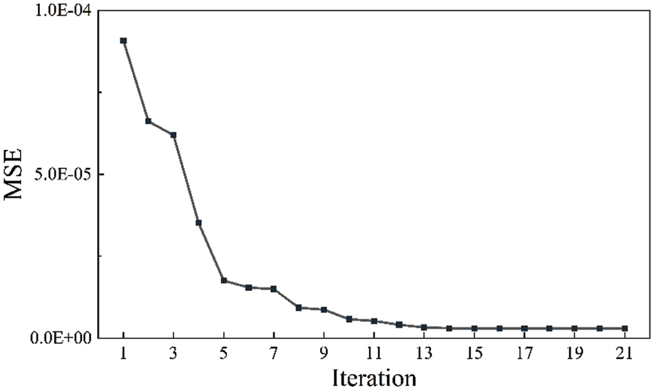
Figure 14: ACO-ANN performance in the training process

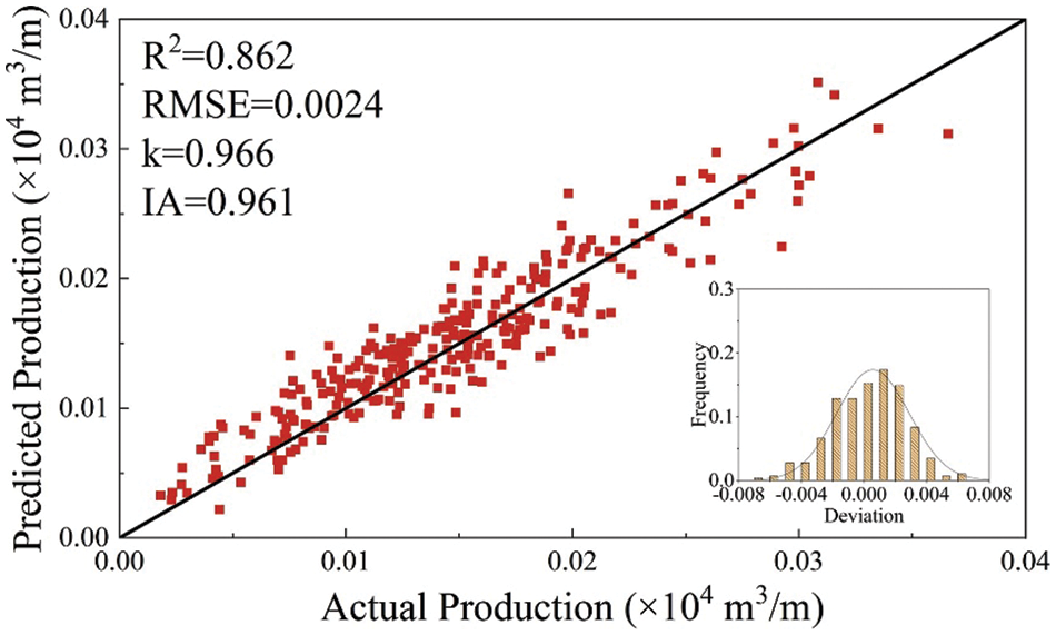
Figure 15: The predictive performance of ACO-ANN model on the training set

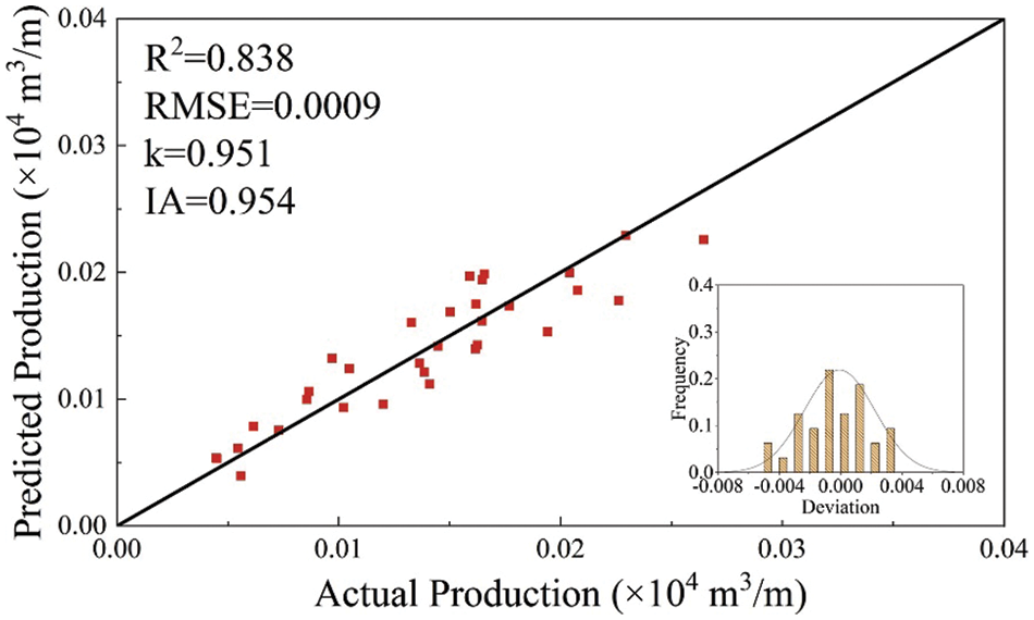
Figure 16: The predictive performance of ACO-ANN model on the testing set

3.4 Comparison and Evaluation of the Developed Models

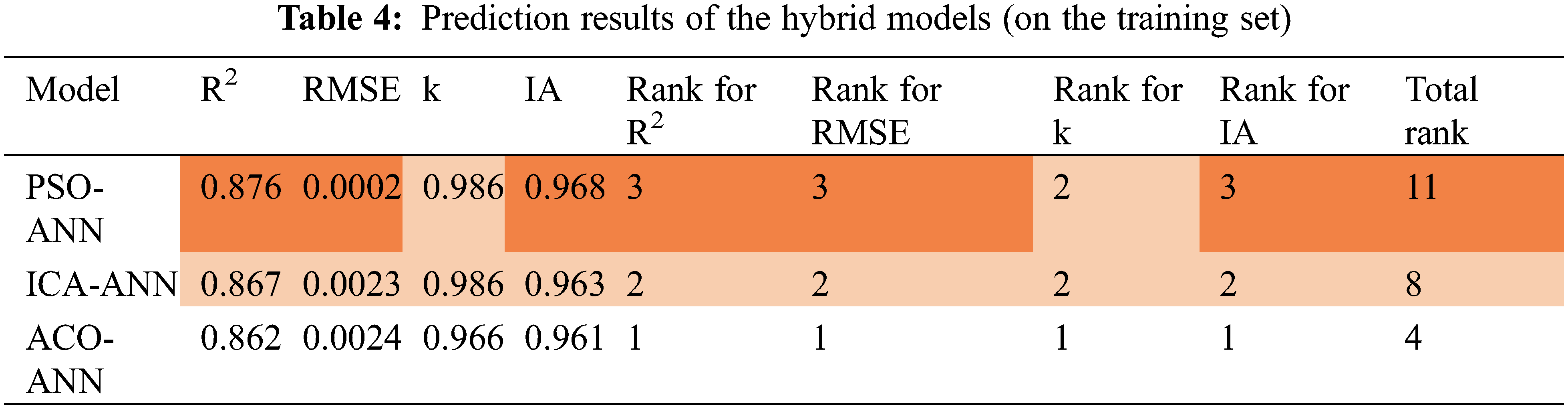
The results of the three developed models were compared through the ranking and intensity of color. From Table 4, the color intensity showed that the performance for predicting shale gas production in the order from dominant to weakest is: PSO-ANN, ICA-ANN, ACO-ANN, with the total ranking of 11, 8, 4, respectively. To have a complete conclusion, the models’ performances were assessed on the testing dataset, where the dataset was considered as the new data and ever not used in the training process.

Based on the reports of Table 5, the color intensity indicated that the PSO-ANN model was the best model with the total ranking of 11. Whereas, the ICA-ANN and ACO-ANN model proved lower performances, as like the training process, with the total ranking of 6 and 5. From the perspective of the four statistical descriptors (R2, RMSE, k, IA), the PSO-ANN model ranks highest and provided the highest performance on both training and testing set (i.e., lowest error).

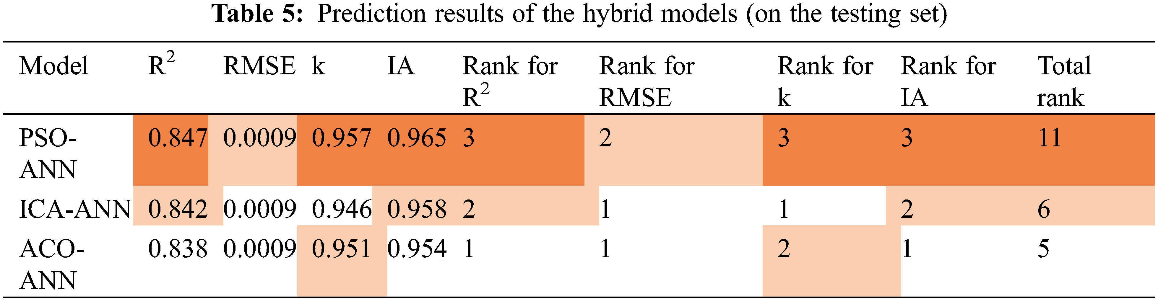
Fig. 17 compared the variation of RMSE with the number of iterations in the three models. In the PSO-ANN model, the RMSE decreased the fastest with the number of iterations, and the minimal RMSE was finally achieved (i.e., highest efficiency). From this perspective, the PSO-ANN model provided the highest performance as well. As can be seen from Figs. 18 and 19, the maximum relative deviation of the PSO-ANN model is observed in the early boundary on both the training and testing set.

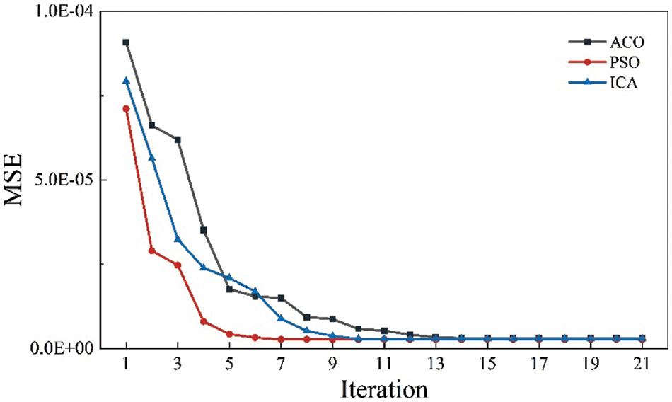
Figure 17: RMSE vs. with the iterations in the three models

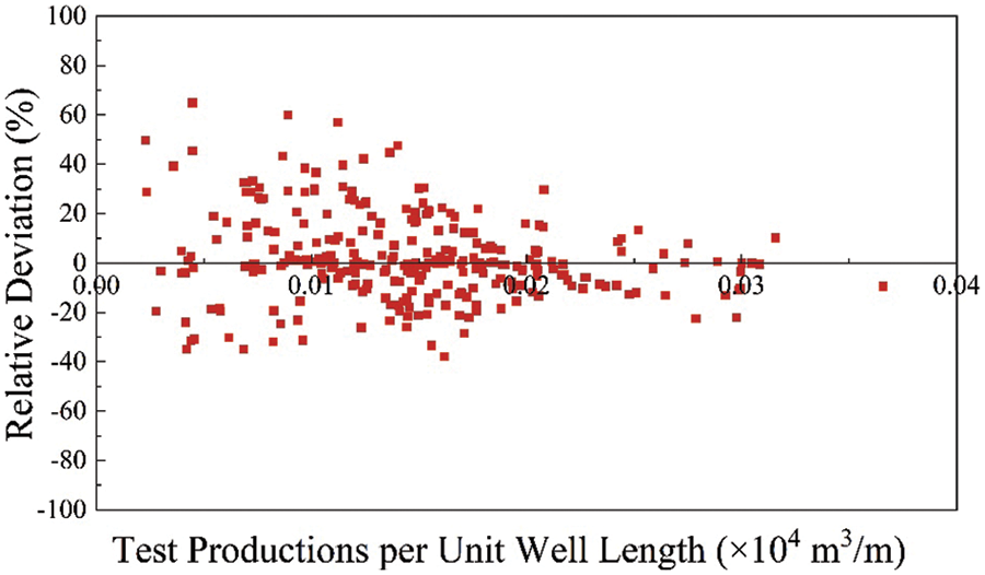
Figure 18: Relative deviation distribution of the PSO-ANN model on training set

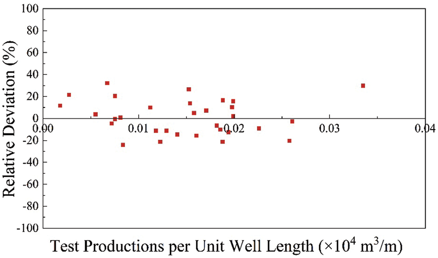
Figure 19: Relative deviation distribution of the PSO-ANN model on training set

3.5 Relative Importance of Influencing Factors

Fig. 20 shows the PDP of the 15 variables in the ANN model affecting the prediction results of shale gas productivity. The relative importance of variables can be determined using the slope of PDP, and the greater the slope, the greater the relative importance as shown in Fig. 21.

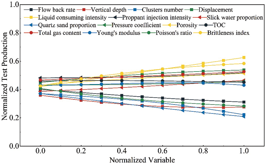
Figure 20: PDP of normalized variable

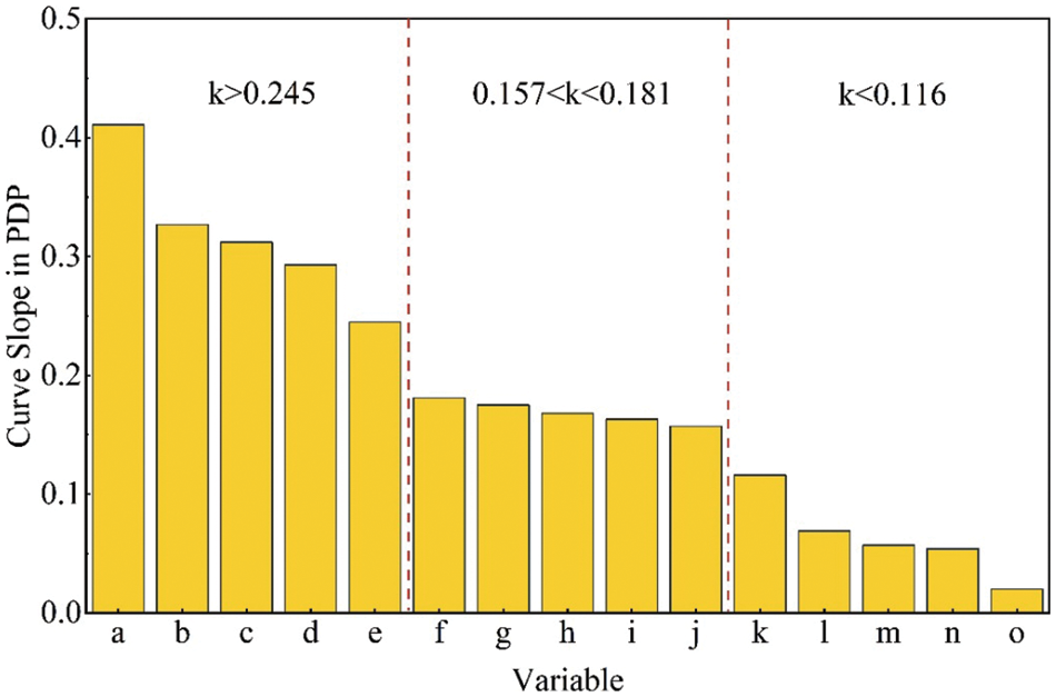
Figure 21: Ranking of relative importance of variables

Results indicated that the order of relative importance of the 15 variables was as follows: liquid consuming intensity > quartz sand proportion > brittleness index> cluster number > Poisson’s ratio > flow back rate > displacement > vertical depth > porosity > slick water proportion > total gas content > proppant injection intensity > Young’s modulus > pressure coefficient > TOC. According to the above order, the corresponding variable serial numbers were a, b, c, d, e, f, g, h, i, j, k, l, m, n, and o.

4  Prospects and Challenges

The main aim of this study was to verify the PSO-ANN method for prediction of shale gas horizontal well production. The PSO-ANN method has the advantages of less time consuming and low cost, which is more obvious in the research with large data samples. In addition, the PSO-ANN method has the following advantages: (1) Accuracy of the PSO-ANN method will not suffer from idealized assumptions and parameter settings, and it can automatically learn and solve the nonlinear relationship between input and output variables using only input variables. (2) The hybrid models can directly predict the test production per unit well length from the influencing variables, without field production testing, that is, there is no need for history matching data in the early stage of horizontal shale gas well drainage. (3) A more comprehensive data set can be used to easily build and update a general model, which indicates that the generalization capability of the hybrid model was good.

Though a large number of scientific studies have proved that the application of ML technology for natural gas production prediction is very promising, there are still challenges. First of all, the dataset came from shale gas wells in China, and the trained model may not be generalized to shale gas wells in other regions because the characterization and fracturing techniques in other reservoirs are different. Thus, a cross regional and highly accessible database is an important prerequisite. How to improve the prediction accuracy is another challenge because advanced algorithms are rare and urgently needed. Lastly, How to apply artificial intelligence technology to other aspects in the shale gas horizontal well fracturing design process is also worth studying.

5  Conclusion

This paper proposed three new artificial intelligence techniques for predicting the shale gas production based on the ANN combined with PSO, ICA, and ACO. Comparison were performed in this work and the relative variable importance was investigated using PDP. According to the results of this study, the following conclusions can be drawn:

(1)The optimum ANN-PSO model constructed for predicting the productivity of shale gas horizontal wells had 1 hidden layer with 69 neurons.

(2)The PSO provided the highest performance in optimizing the ANN model. The predicting performance that IA = 0.965, k = 0.957, RMSE = 0.0009 and R2 = 0.847. The ANN-PSO model optimized was successful in learning the nonlinear relationship between shale gas production and variables affecting the prediction.

(3)PDP indicated that liquid consuming intensity and the proportion of quartz sand are the two most sensitive factors affecting the accuracy of the optimum ANN-PSO model’s performance predicting the productivity of shale gas horizontal wells.

Funding Statement: This study was financially supported by China United Coalbed Methane Corporation, Ltd. (ZZGSSALFGR2021-581), Bin Li received the grant.

Author Contributions: Bin Li studied conception and design, collected data, analysis results, drafted manuscript preparation, reviewed the results and approved the final version of the manuscript.

Conflicts of Interest: The author declare that he has no conflicts of interest to report regarding the present study.

References

1. Aziz, K., Arbabi, S., Deutsch, C. V. (1999). Why is it so difficult to predict the performance of horizontal wells? Journal of Canadian Petroleum Technology, 38(10), 37–45. [Google Scholar]

2. Peng, Y., Zhao, J., Sepehrnoori, K., Li, Z. (2020). Fractional model for simulating the viscoelastic behavior of artificial fracture in shale gas. Engineering Fracture Mechanics, 228, 106892. [Google Scholar]

3. Jia, A. (2018). Progress and prospects of natural gas development technologies in China. Natural Gas Industry B, 5(6), 547–557. [Google Scholar]

4. Zhao, J., Ren, L., Jiang, T., Hu, D., Wu, L. et al. (2022). Ten years of gas shale fracturing in China: Review and prospect. Natural Gas Industry B, 9(2), 158–175. [Google Scholar]

5. Fang, B., Hu, J., Xu, J., Zhang, Y. (2020). A semi-analytical model for horizontal-well productivity in shale gas reservoirs: Coupling of multi-scale seepage and matrix shrinkage. Journal of Petroleum Science and Engineering, 195, 107869. [Google Scholar]

6. Zheng, D., Miska, S., Ziaja, M., Zhang, J. (2019). Study of anisotropic strength properties of shale. AGH Drilling, Oil, Gas, 36(1), 93–112. [Google Scholar]

7. Li, Z., Peng, Y., Peng, H. (2022). Simulation of borehole shrinkage in shale based on the triaxial fractional constitutive equation. Geomechanics and Geophysics for Geo-Energy and Geo-Resources, 8(2), 65. [Google Scholar]

8. Jia, C., Zhang, Y., Zhao, X. (2014). Prospects of and challenges to natural gas industry development in China. Natural Gas Industry B, 1(1), 1–13. https://doi.org/10.1016/j.ngib.2014.10.001 [Google Scholar] [CrossRef]

9. Li, T., Li, C. (2005). The electrolytic simulation experiment research of fractured horizontal well’s productivity in low permeability reservoirs. China Offshore Oil and Gas, 17(6). [Google Scholar]

10. Pei, B., Huang, D., Liu, Y. (2003). Horizontal well physical model and simulating test. Oil Drilling & Production Technology, 25(6), 50–53. [Google Scholar]

11. Cheng, Y., Dong, B., Shi, X., Li, N., Yuan, Z. (2012). Seepage mechanism of three-hole double-permeability model in shale gas reservoir. Natural Gas Industry, 32(9), 44–47. [Google Scholar]

12. Yu, W., Zhang, T., Du, S., Sepehrnoori, K. (2015). Numerical study of the effect of uneven proppant distribution between multiple fractures on shale gas well performance. Fuel, 142(4), 189–198. [Google Scholar]

13. Chen, X., Li, J., Gao, P., Zhou, J. (2022). Prediction of shale gas horizontal wells productivity after volume fracturing using machine learning—An LSTM approach. Petroleum Science and Technology, 40(15), 1861–1877. [Google Scholar]

14. Tian, J., Chen, C., Qin, Y., Kang, N. (2022). Pore-scale systematic study on the disconnection of bulk gas phase during water imbibition using visualized micromodels. Physics of Fluids, 34(6), 062015. [Google Scholar]

15. Zhao, J., Peng, Y., Li, Y., Tian, Z. (2017). Applicable conditions and analytical corrections of plane strain assumption in the simulation of hydraulic fracturing. Petroleum Exploration and Development, 44(3), 454–461. [Google Scholar]

16. Hu, Y., Peng, X., Li, Q. (2020). Progress and development direction of technologies for deep marine carbonate gas reservoirs in the Sichuan Basin. Natural Gas Industry B, 7(2), 149–159. [Google Scholar]

17. He, J., Jiang, R., Sun, J., Gao, Y. (2016). Multi-stage fractured horizontal well productivity evaluation in shale gas reservoir. Special Oil & Gas Reservoirs, 23(4), 96–100. [Google Scholar]

18. Jia, C., Jia, A., He, D., Wei, Y., Qi, Y. et al. (2017). Key factors influencing shale gas horizontal well production. Natural Gas Industry, 37(4), 80–88. [Google Scholar]

19. Yu, W., Tan, X., Zuo, L., Liang, J. (2016). A new probabilistic approach for uncertainty quantification in well performance of shale gas reservoirs. SPE Journal, 21(6), 2038–2048. [Google Scholar]

20. Gong, X., Gonzalez, R., Mcvay, D. A., Hart, J. (2014). Bayesian probabilistic decline-curve analysis reliably quantifies uncertainty in shale-well-production forecasts. SPE Journal, 19(6), 1047–1057. [Google Scholar]

21. Guo, Z., Zhao, J., You, Z., Li, Y., Zhang, S. et al. (2021). Prediction of coalbed methane production based on deep learning. Energy, 230(2), 120847. [Google Scholar]

22. Moosavi, S. R., Wood, D. A., Ahmadi, M. A., Choubineh, A. (2019). ANN-based prediction of laboratory-scale performance of CO2-foam flooding for improving oil recovery. Natural Resources Research, 28(4), 1–9. [Google Scholar]

23. Syed, F. I., Dahaghi, A. K., Muther, T. (2022). Laboratory to field scale assessment for EOR applicability in tight oil reservoirs. Petroleum Science, 19(5), 2131–2149. [Google Scholar]

24. Le, L. T., Nguyen, H., Dou, J., Zhou, J. (2019). A comparative study of PSO-ANN, GA-ANN, ICA-ANN, and ABC-ANN in estimating the heating load of buildings’ energy efficiency for smart city planning. Applied Sciences, 9(13), 2630. [Google Scholar]

25. Rukhaiyar, S., Alam, M. N., Samadhiya, N. K. (2018). A PSO-ANN hybrid model for predicting factor of safety of slope. International Journal of Geotechnical Engineering, 12(6), 556–566. [Google Scholar]

26. Xu, C., Shen, P., Yang, Y. (2014). Accumulation conditions and enrichment patterns of natural gas in the Lower Cambrian Longwangmiao Fm reservoirs of the Leshan-Longnǚsi Palaeohigh, Sichuan Basin. Natural Gas Industry B, 1(1), 51–57. [Google Scholar]

27. Lin, B., Guo, J., Liu, X., Xiang, J., Zhong, H. (2019). Prediction of flowback ratio and production in Sichuan shale gas reservoirs and their relationships with stimulated reservoir volume. Journal of Petroleum Science and Engineering, 184(3), 106529. [Google Scholar]

28. Wang, S., Chen, Z., Chen, S. (2019). Applicability of deep neural networks on production forecasting in Bakken shale reservoirs. Journal of Petroleum Science and Engineering, 179(49), 112–125. [Google Scholar]

29. Ramdya, P., Thandiackal, R., Cherney, R., Asselborn, T., Benton, R. et al. (2017). Climbing favours the tripod gait over alternative faster insect gaits. Nature Communications, 8(1), 14494. [Google Scholar] [PubMed]

30. Ahmadi, M. A. (2011). Prediction of asphaltene precipitation using artificial neural network optimized by imperialist competitive algorithm. Journal of Petroleum Exploration and Production Technology, 1(2–4), 99–106. [Google Scholar]

31. Ahmadi, M. A., Ebadi, M., Shokrollahi, A., Majidi, S. M. J. (2013). Evolving artificial neural network and imperialist competitive algorithm for prediction oil flow rate of the reservoir. Applied Soft Computing Journal, 13(2), 1085–1098. [Google Scholar]

32. Friedman, J. H. (2001). Greedy function approximation: A gradient boosting machine. Annals of Statistics, 29(5), 1189–1232. [Google Scholar]

33. Wang, H., Shi, Z., Sun, S., Zhang, L. (2021). Characterization and genesis of deep shale reservoirs in the first Member of the Silurian Longmaxi Formation in Southern Sichuan Basin and its periphery. Oil & Gas Geology, 42(1), 66–75. [Google Scholar]

34. Peng, Y., Zhao, J., Sepehrnoori, K. (2019). Study of the heat transfer in wellbore during acid/hydraulic fracturing based on semi-analytical transient model. SPE Journal, 24(2), 877–890. [Google Scholar]

35. Zhou, S., Zhao, J., Li, Q. (2018). Optimal design of the engineering parameters for the first global trial production of marine natural gas hydrates through solid fluidization. Natural Gas Industry B, 5(2), 118–131. [Google Scholar]

36. Mustafa, A., Tariq, Z., Mahmoud, M. (2022). Data-driven machine learning approach to predict mineralogy of organic-rich shales: An example from Qusaiba Shale, Rub’al Khali Basin, Saudi Arabia. Marine and Petroleum Geology, 137(5), 105495. [Google Scholar]

37. Radwan, A. E., Wood, D. A., Radwan, A. A. (2022). Machine learning and data-driven prediction of pore pressure from geophysical logs: A case study for the Mangahewa gas field, New Zealand. Journal of Rock Mechanics and Geotechnical Engineering, 14(6), 1799–1809. [Google Scholar]

38. Jafarizadeh, F., Rajabi, M., Tabasi, S. (2022). Data driven models to predict pore pressure using drilling and petrophysical data. Energy Reports, 8(3568), 6551–6562. [Google Scholar]

39. Manzoor, U., Ehsan, M., Radwan, A. E. (2023). Seismic driven reservoir classification using advanced machine learning algorithms: A case study from the lower Ranikot/Khadro sandstone gas reservoir, Kirthar fold belt, lower Indus Basin. Pakistan Geoenergy Science and Engineering, 222, 211451. [Google Scholar]

40. Wang, Y., Dong, D., Li, J., Wang, S., Li, X. et al. (2012). Reservoir characteristics of shale gas in Longmaxi Formation of the Lower Silurian, Southern Sichuan. Acta Petrolei Sinica, 33(4), 551–561. [Google Scholar]

41. Peng, Y., Zhao, J., Sepehrnoori, K. (2019). Study of delayed creep fracture initiation and propagation based on semi-analytical fractional model. Applied Mathematical Modelling, 72, 700–715. [Google Scholar]

42. Guo, X., Hu, D., Huang, R. (2020). Deep and ultra-deep natural gas exploration in the Sichuan Basin: Progress and prospect. Natural Gas Industry B, 7(5), 419–432. [Google Scholar]

43. Tang, X. (2014). Elements of the sweet spot and their influence on shale oil and gas. School of Geosciences, Yangtze University, China. [Google Scholar]

44. Wu, Q., Liang, X., Xian, C., Liu, X. (2015). Geoscience-to-production integration ensures effective and efficient South China marine shale gas development. China Petroleum Exploration, 20(4), 1–23. [Google Scholar]

45. Peng, Y., Zhao, J., Sepehrnoori, K., Li, Y., Li, Z. (2020). The influences of stress level, temperature, and water content on the fitted fractional orders of geomaterials. Mechanics of Time-Dependent Materials, 24(2), 221–232. [Google Scholar]

46. Zou, C., Zhao, Q., Chen, J., Li, J., Yang, Z. et al. (2018). Natural gas in China: Development trend and strategic forecast. Natural Gas Industry B, 5(4), 380–390. [Google Scholar]

47. Wang, W., Yao, J., Zeng, Q., Sun, H., Fan, D. (2016). Numerical modeling of staged cluster fracturing and gas flow in horizontal wells of shale gas reservoirs. Science Technology and Engineering, 16(14), 160–165. [Google Scholar]

48. Hu, Y., Peng, Y. (2017). Electrochemical analysis of the corrosion behavior of drill pipe steel under oil/water emulsion condition. International Journal of Electrochemical Science, 12, 8526–8534. [Google Scholar]

49. Rajabi, M., Beheshtian, S., Davoodi, S. (2021). Novel hybrid machine learning optimizer algorithms to prediction of fracture density by petrophysical data. Journal of Petroleum Exploration and Production Technology, 11(12), 4375–4397. [Google Scholar]

50. Zhang, F., Wu, J., Huang, H., Wang, X., Luo, H. et al. (2021). Technological parameter optimization for improving the complexity of hydraulic fractures in deep shale reservoirs. Natural Gas Industry, 41(1), 125–135. [Google Scholar]

51. Zhang, T., Li, X., Yang, L., Li, J., Wang, Y. et al. (2017). Effects of shut-in timing on flowback rate and productivity of shale gas wells. Natural Gas Industry, 37(8), 48–60. [Google Scholar]

52. Hu, Y., Peng, Y. (2017). Anti-corrosion performance of chromium-coated steel in a carbon dioxide-saturated simulated oilfield brine. International Journal of Electrochemical Science, 12, 5628–5635. [Google Scholar]

53. Wang, X., Lin, Y., Miu, W. (2021). Volume fracturing technology of deep shale gas in Southern Sichuan. Petroleum Reservoir Evaluation and Development, 11(1), 102–108. [Google Scholar]

54. Cao, H., Zhan, G., Yu, X., Zhao, Y. (2019). The main factors affecting the productivity of deep shale gas wells: Taking the Yongchuan block in the Southern Sichuan Basin as an example. Natural Gas Industry, 39(S1), 118–122. [Google Scholar]

55. Zeng, B., Wang, X., Huang, H., Zhang, N., Yue, W. (2020). Key technology of volumetric fracturing in deep shale gas horizontal wells in Southern Sichuan. Petroleum Drilling Techniques, 48(5), 77–84. [Google Scholar]

56. Li, Y., Liao, Y., Zhao, J. (2017). Simulation and analysis of wormhole formation in carbonate rocks considering heat transmission process. Journal of Natural Gas Science and Engineering, 42(1), 120–132. [Google Scholar]

57. Zheng, X., Wang, X., Zhang, F., Yang, N., Cai, B. et al. (2021). Domestic sand proppant evaluation and research progress of sand source localization and its prospects. China Petroleum Exploration, 26(1), 131–137. [Google Scholar]

58. Roy, P. P., Roy, K. (2008). On some aspects of variable selection for partial least squares regression models. QSAR & Combinatorial Science, 27(3), 302–313. [Google Scholar]